Introduction to eDNA & Biodiversity Data
What is eDNA?
Environmental DNA (eDNA) is, in the words of the researcher who coined the term:
“Any DNA collected from an environmental sample without first isolating the target organisms.” — Taberlet, 2012
In practice, that means: instead of catching, netting, or observing an organism directly, you collect a sample of water, soil, sediment, or even air, and extract whatever DNA happens to be in it. That DNA can come from:
- Free-floating DNA released into the water
- DNA bound to particles
- Whole cells, organelles, or fragments of tissue (mucus, scales, faeces, skin)
It can belong to anything from viruses and bacteria to fish, crustaceans, and plants. This is what makes eDNA so powerful for biodiversity monitoring: a single water sample can reveal the presence of dozens of species, including ones that are cryptic, rare, or otherwise very difficult to observe directly — without ever disturbing the animal itself.
Two data types come up most often in eDNA work, and this training focuses on the first:
- Metabarcoding — detects many taxa at once from a single sample
- Quantitative PCR (qPCR) — targets one specific species or small group, and can estimate how much of its DNA is present
What is eDNA metabarcoding?
The name breaks down into two parts:
- Barcoding — identifying a species using a short, standardized genetic marker sequence, much like a supermarket barcode identifies a product.
- Meta — doing this for everything in the sample at once, rather than one organism at a time.
Put together, metabarcoding amplifies and sequences a shared genetic marker from every organism present in a sample simultaneously, then works out afterwards which sequences belong to which taxa.
Not all genetic markers are equal. The choice of marker determines which organisms can even be detected, and there’s always a trade-off between how broad a group you can capture and how precisely you can resolve species within it. Common markers include 12S and 16S (often for vertebrates/prokaryotes), 18S (broad eukaryotes), COI (animals), and ITS (fungi).
The metabarcoding workflow
An eDNA metabarcoding study generally moves through six stages, from a bottle of water to a table of species detections:
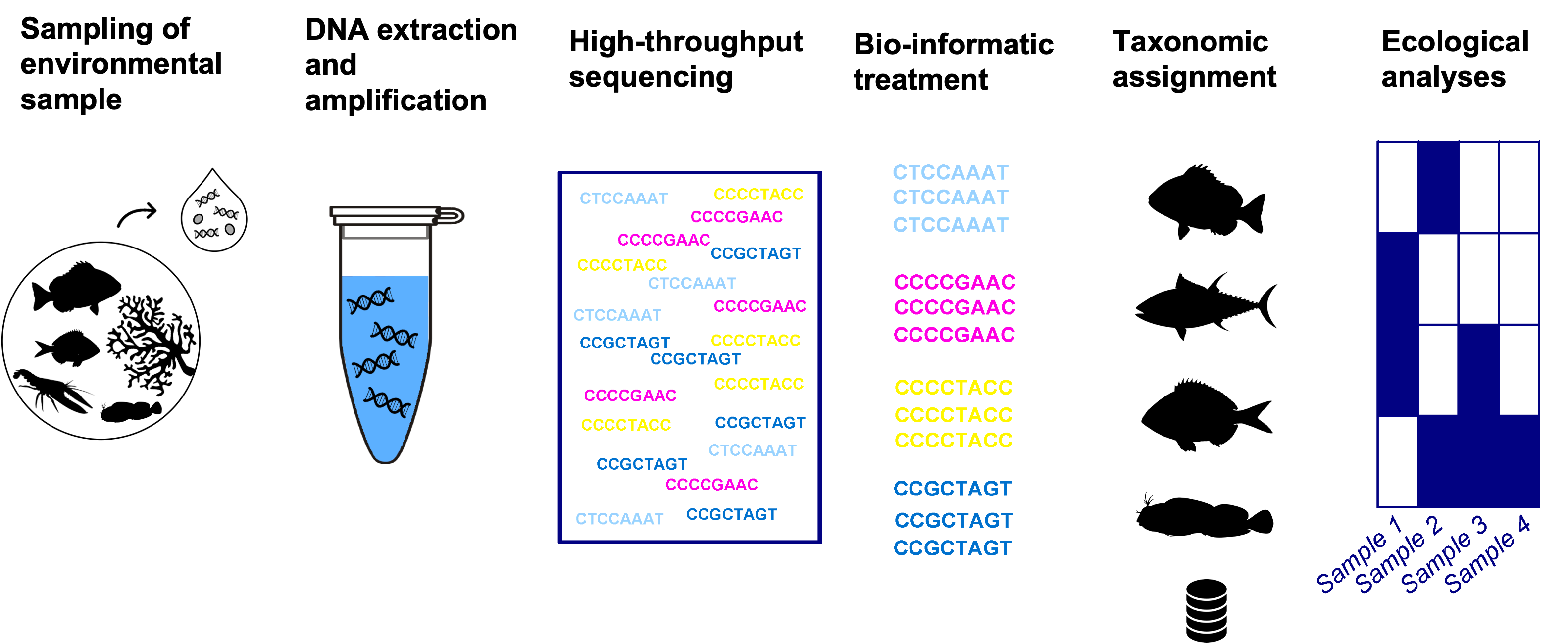
- Sample collection — water, soil, or sediment is collected in the field.
- DNA extraction and PCR amplification — DNA is extracted from the sample, and the chosen marker is amplified using specific primers.
- High-throughput sequencing — modern sequencers read millions of DNA fragments from the sample simultaneously.
- Bioinformatic treatment — reads are quality-filtered and clustered into Operational Taxonomic Units (OTUs) or Amplicon Sequence Variants (ASVs) — in practice, “the distinct sequences found in this sample.”
- Taxonomic assignment — each OTU/ASV is compared against a reference database to assign it a taxon name.
- Ecological analysis — the result is a presence/absence (or abundance) matrix of taxa across samples, ready for ecological interpretation.
This is exactly the shape of the raw files you’ll work with hands-on in Episode 4: an ASV table (step 4), a taxonomy table (step 5), and sample metadata (step 1) — the building blocks of one eDNA dataset.
Metabarcoding vs. qPCR
| Metabarcoding | qPCR | |
|---|---|---|
| Question answered | “What’s in this sample?” | “Is species X in this sample, and how much?” |
| Output | Many taxa, presence/read count | One (or a few) targeted taxa, with a quantity estimate |
| Typical use | Broad biodiversity surveys | Early detection of invasive or rare/endangered species |
Both are valid, complementary approaches — which one you use depends on the question you’re trying to answer.
Why is eDNA data “special”?
eDNA has enormous potential to expand access to biodiversity data at scale, and raw sequences are already widely shared through NCBI/GenBank. But NCBI alone is not enough:
- Raw sequences deposited there cannot be searched by species, in time, or in space.
- There is no link to spatial coordinates or a sampling date.
- As a result, they cannot support distribution maps, trend analyses, or Marine Protected Area assessments.
On top of that, eDNA data requires extra care for a few reasons that don’t apply to a simple “I saw this animal here” observation:
- ⚗️ It’s derived information, not a direct observation — it passes through extensive laboratory and bioinformatic processing before it becomes a “detection.”
- 📚 It relies on reference databases — your results are only as good as the completeness of the database used for taxonomic assignment.
- ❓ A large fraction of sequences often have no match in any database — this is normal, not a failure, and those sequences still matter.
- 📋 Because of all this, it’s important to record how the detection was made — which is exactly what the Darwin Core DNA extension you’ll meet in the next episode is designed to capture, so the work can be understood and re-analyzed later as reference databases improve.
This is why OBIS, GBIF, and similar biodiversity platforms accept DNA-derived occurrences that are explicitly linked to space and time, rather than treating raw sequence archives as sufficient on their own.
The data standards landscape
Two major standards show up repeatedly when working with eDNA data, and it’s worth knowing the difference before diving deeper:
- MIxS (Minimum Information about any (x) Sequence) — the standard used for describing raw sequences, e.g. when submitting to NCBI/GenBank. It focuses on sequencing and laboratory methods.
- Darwin Core (DwC) — the community vocabulary used for biodiversity data more broadly: species, location, date, basis of record.
For eDNA data to be genuinely useful for biodiversity science, it needs both: the methodological detail from MIxS and the “what, where, when” from Darwin Core. That’s exactly what the Darwin Core DNA Derived Data extension — the subject of the next two episodes — combines into a single publishable format.
This is a rapidly changing field. Future directions for OBIS include newer frameworks like the Darwin Core Data Package (DwC-DP) and FAIReDNA terms. What you’ll learn in this training reflects current best practice, but expect the tooling to keep evolving.