The main gateway to explore the species range maps of the MPA Europe project is the Shiny application (https://shiny.obis.org/distmaps/). It provides an interactive experience, with full access to all species, models and predictions. It also includes important details like the model metrics and partial response curves, helping users to more carefully evaluate the model quality and its uncertainty. Users can also directly download results and reports.
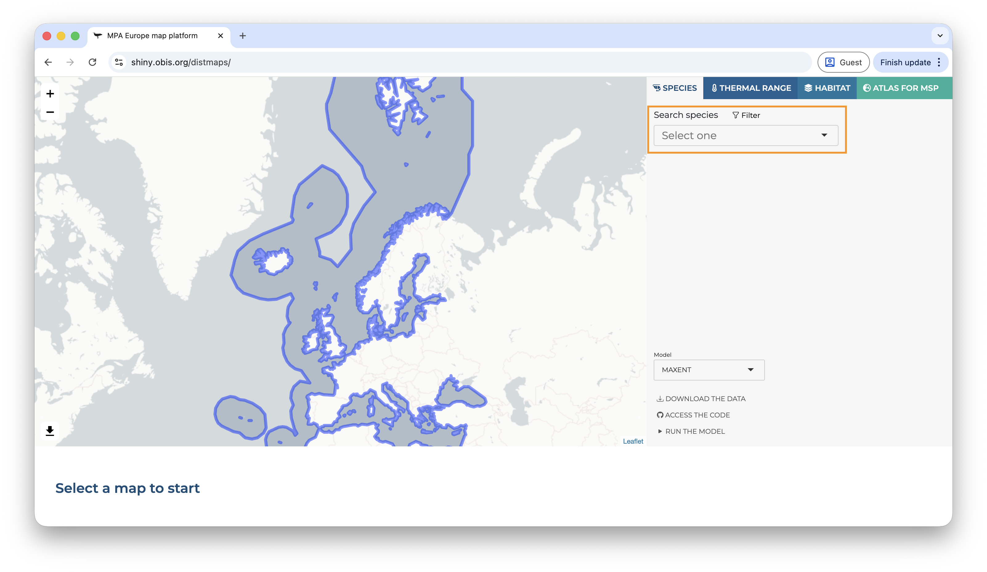
Once you access the application, you will land in a page like that:
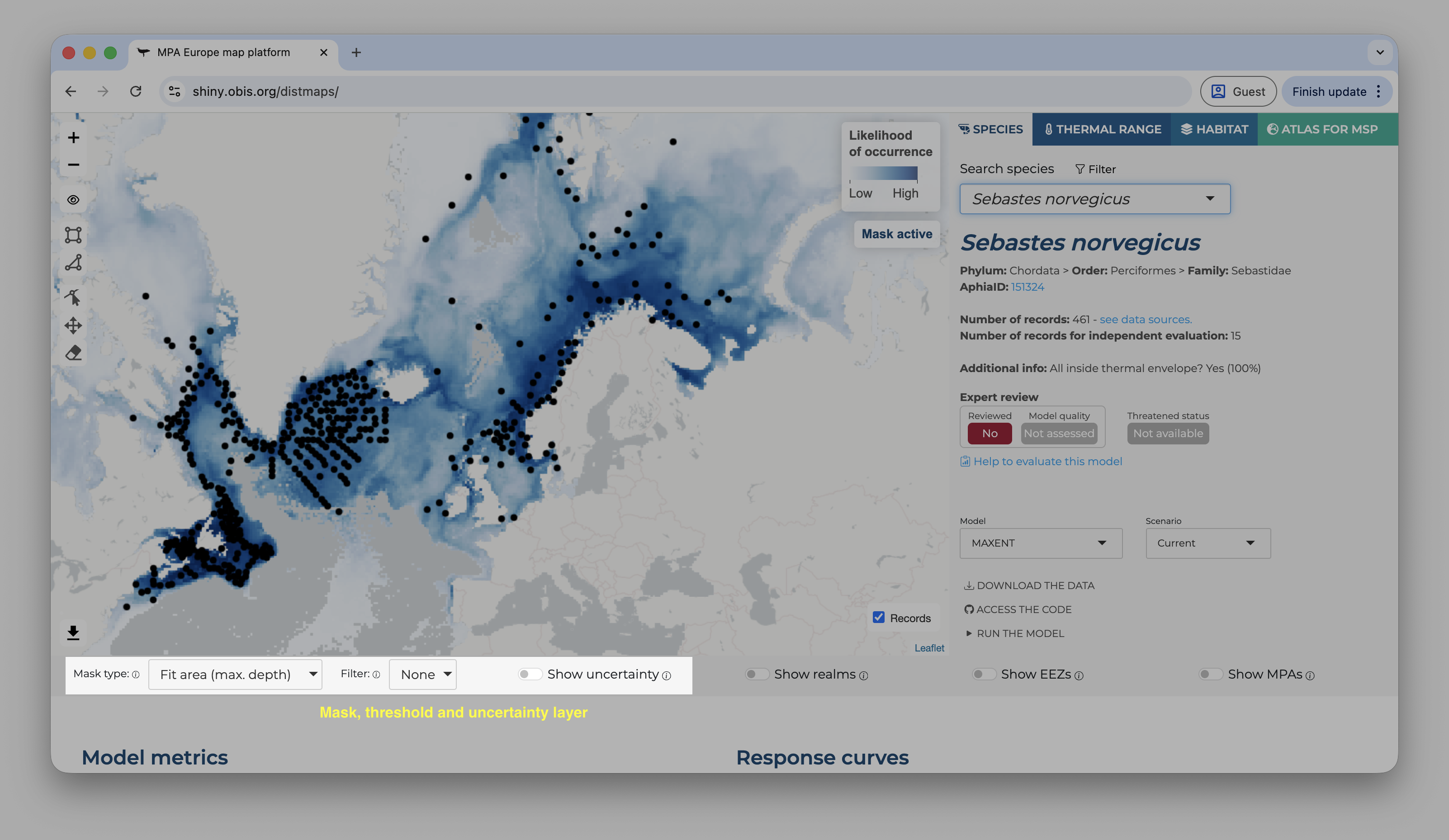
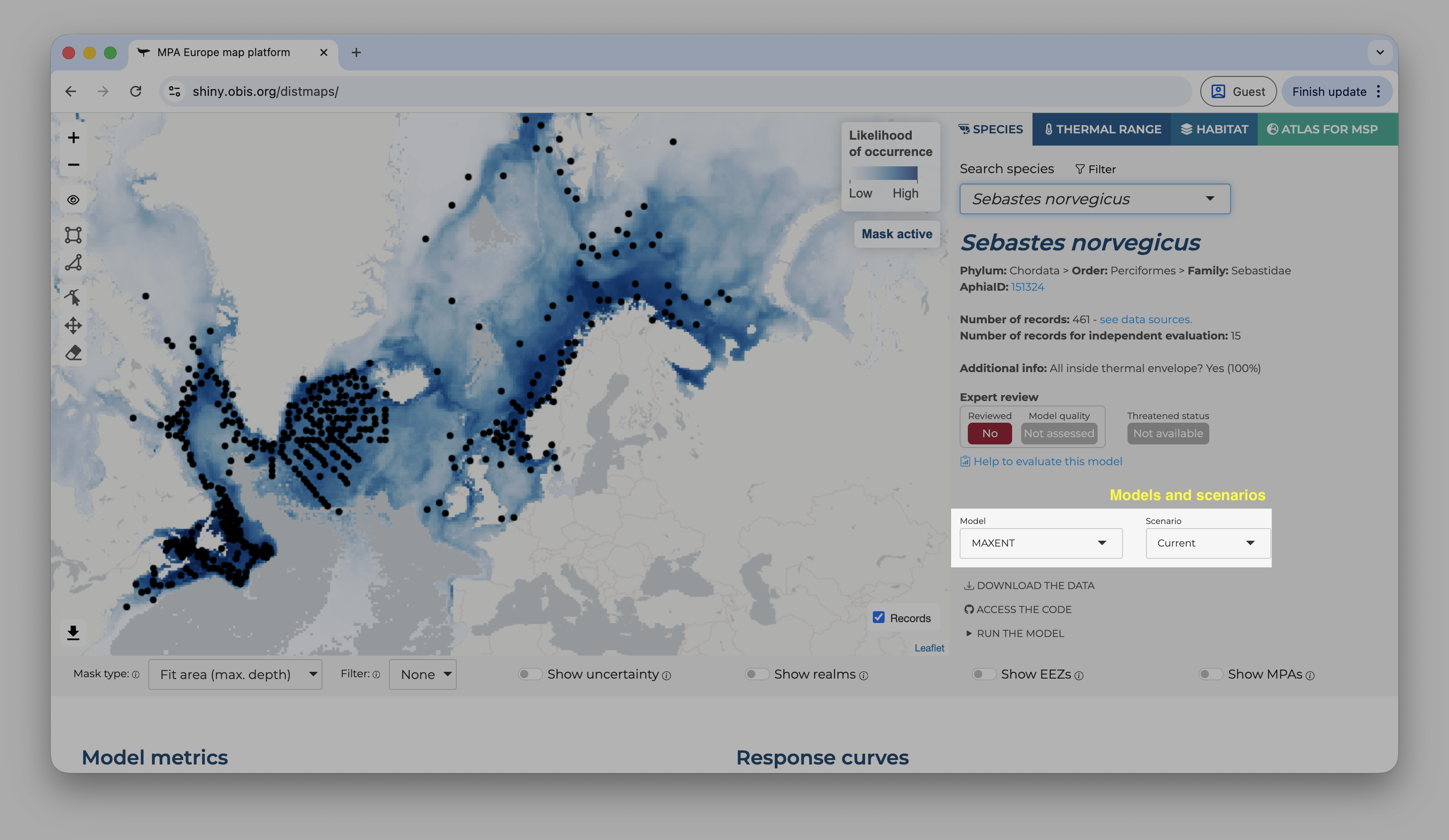
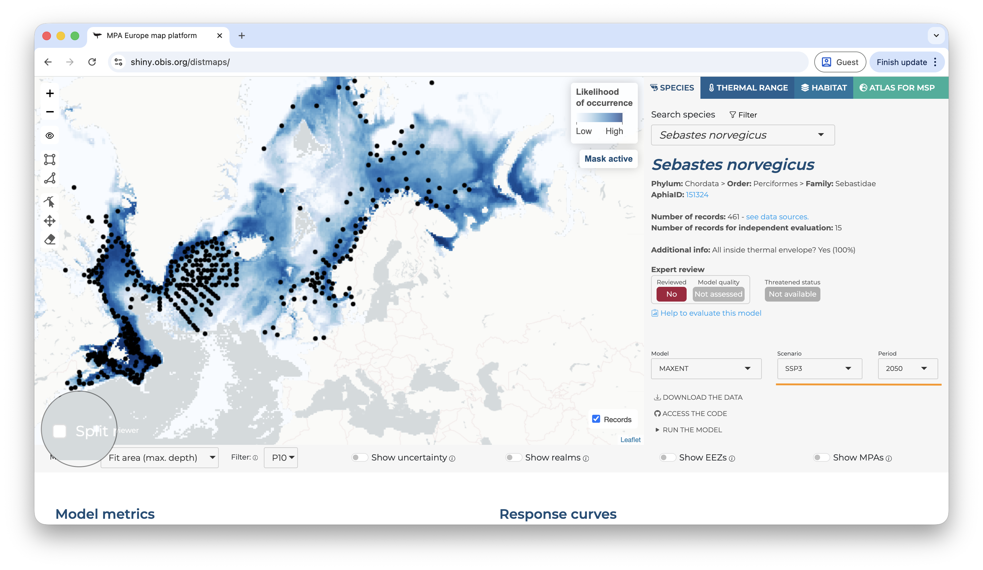
Landing page of the Shiny application
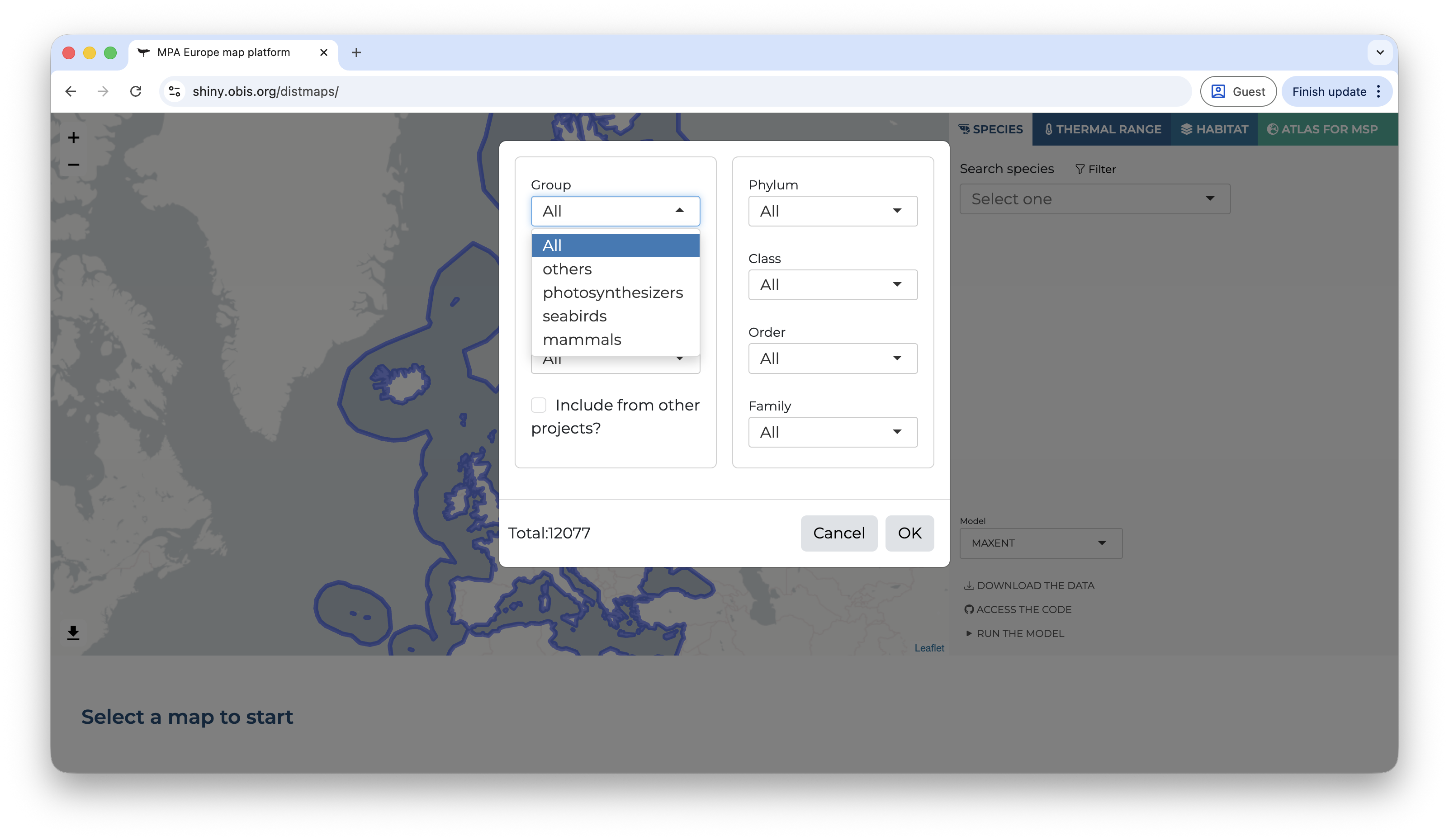
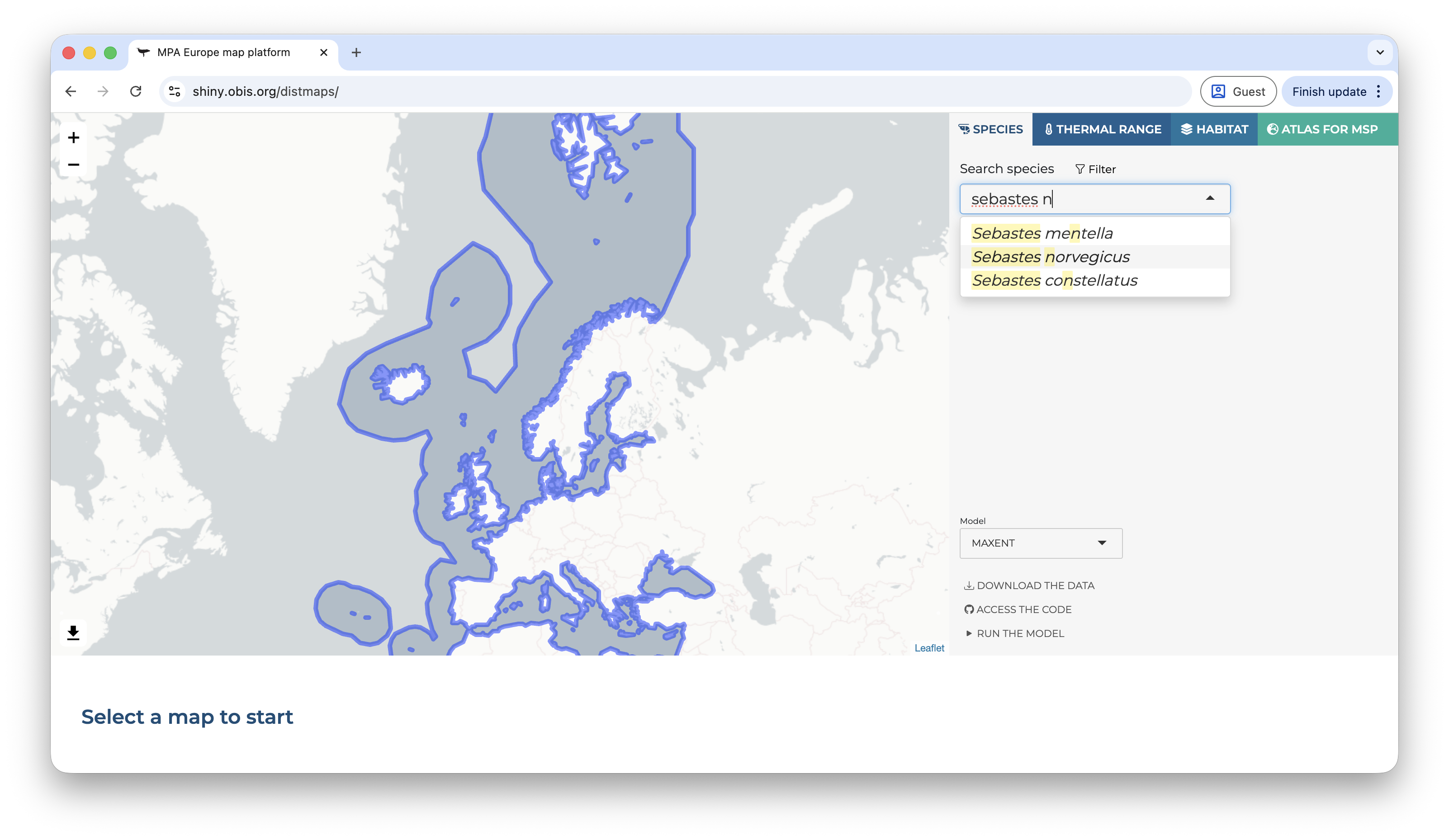
On the top, the user can choose between four tabs. The first show the species range maps, the second species thermal ranges (estimated from the occurrence records), the third the habitat models (based on Stacked SDMs), and the fourth gives access to the Atlas for MSP. On the species tab, the user can type scientific names or use the filter option to limit the search to specific groups/areas of interest.
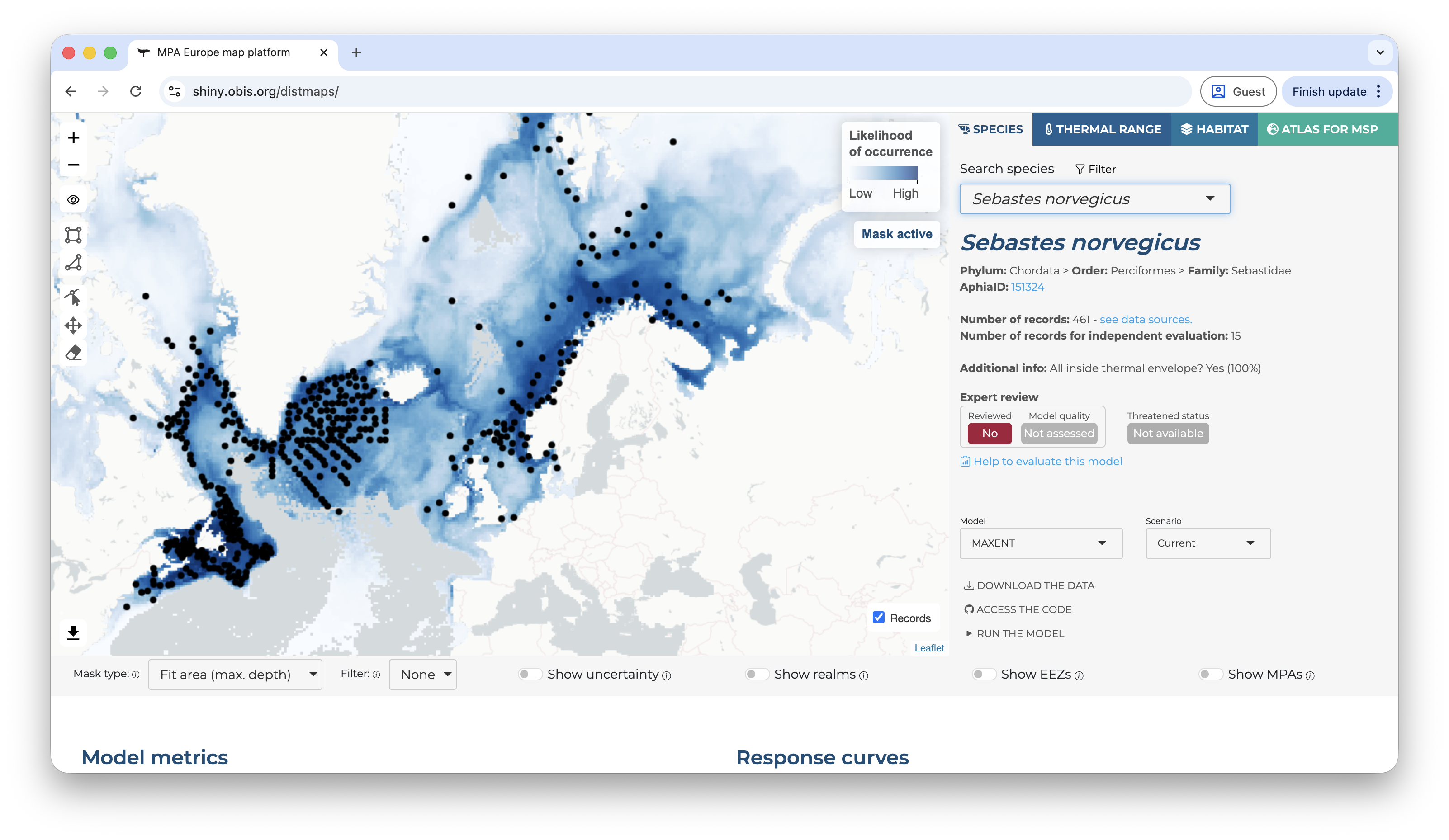
Once a species is selected, a set of new options become available. The first shown map is always for the current period and, by default, mask the prediction by the area used to fit the model limited to the maximum depth where the species was observed1. It is possible do activate or deactivate the mask by clicking on the “eye” symbol on the left panel, over the map. The occurrence records used to fit the model are also shown by default, but can be deactivated by clicking on the “records” button on the bottom-right of the map.
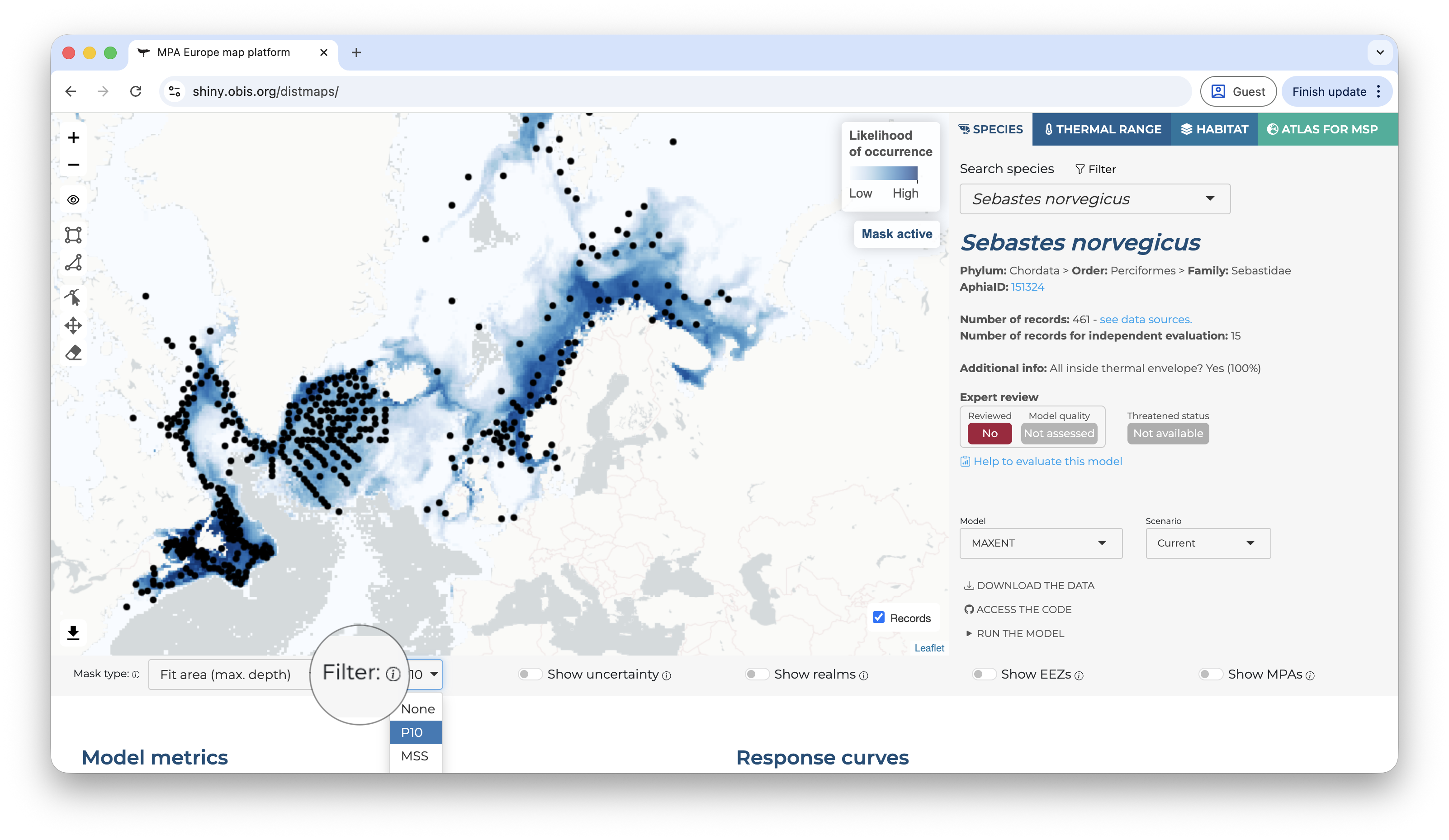
Below the map, on the left side, you will find the options to change the mask type, apply a threshold (under the “filter” option), and also to show the uncertainty map instead (the bootstrap result).
Applying a threshold will automatically update the map, removing areas of low suitability according to the selected threshold.
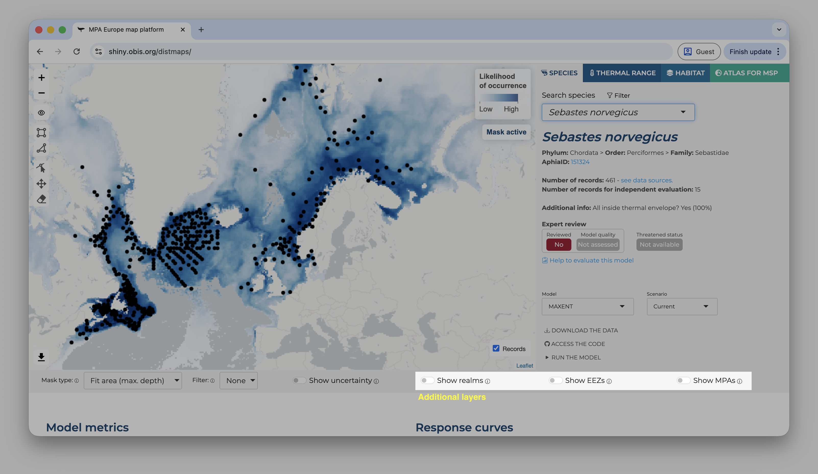
On the right side, it is possible to overlay some additional layers to provide context to the map.
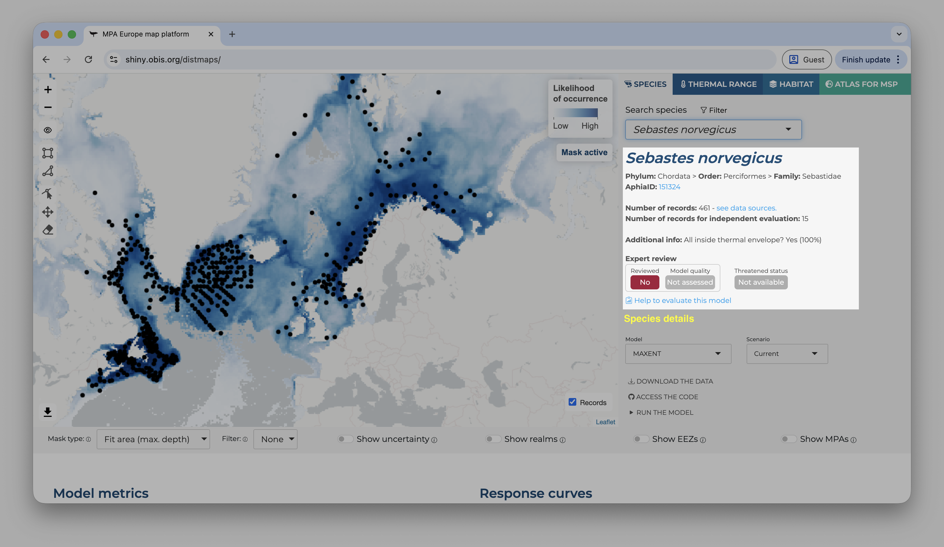
On the right panel, details about the species are available, including it threatened status according to the IUCN Red List and, if available, the expert review.
Right below the species details you will find the control to select the model and the time period of the predictions.
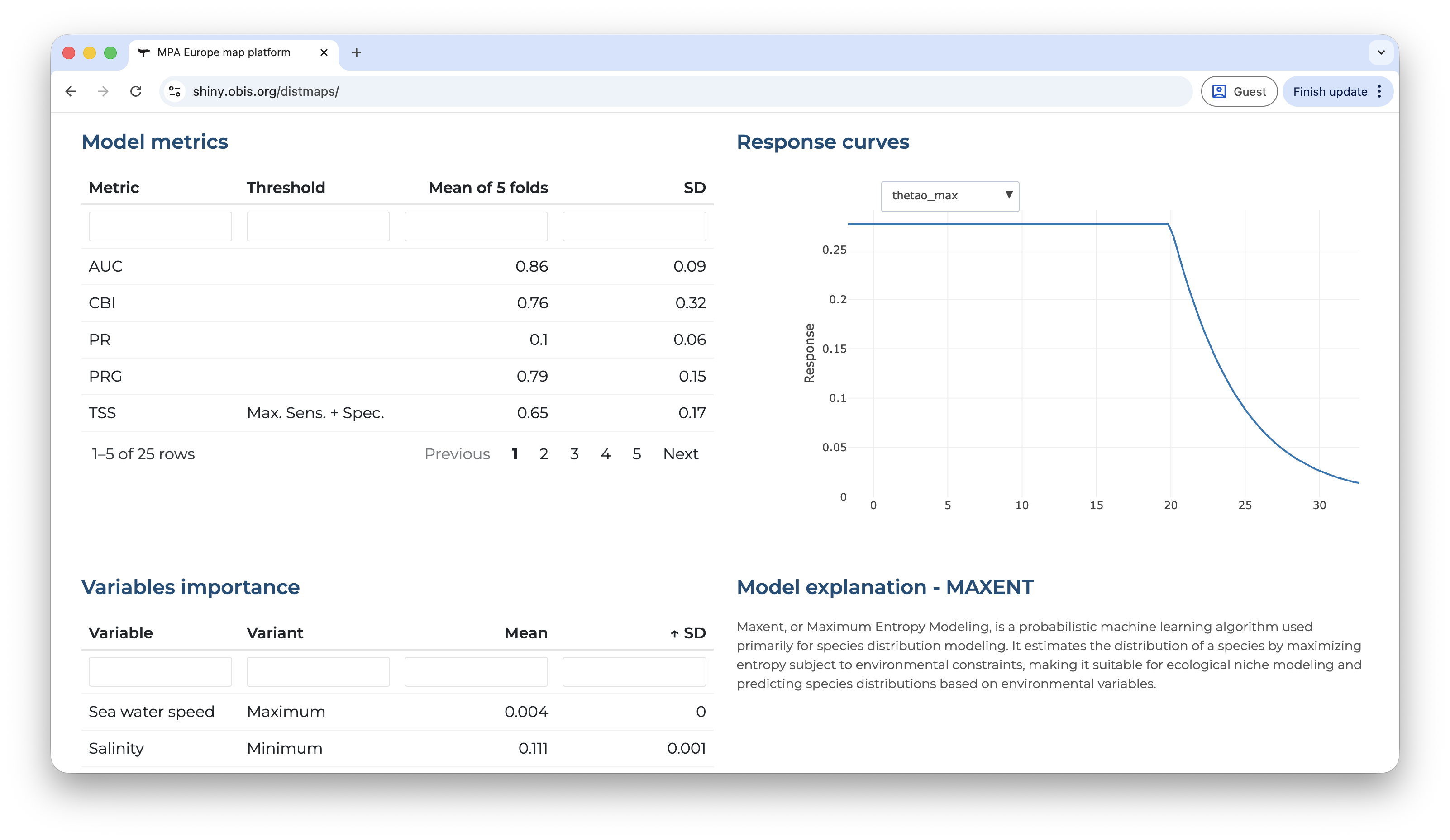
Scrolling-down you will have access to the model metrics, variable importance, the explanation of the selected model and the partial response curves. All of those are extremelly important to enable you to critically evaluate the model. Does the metrics indicate that the model has a good capacity of prediction? The partial response curves show patterns that are biologically plausible?
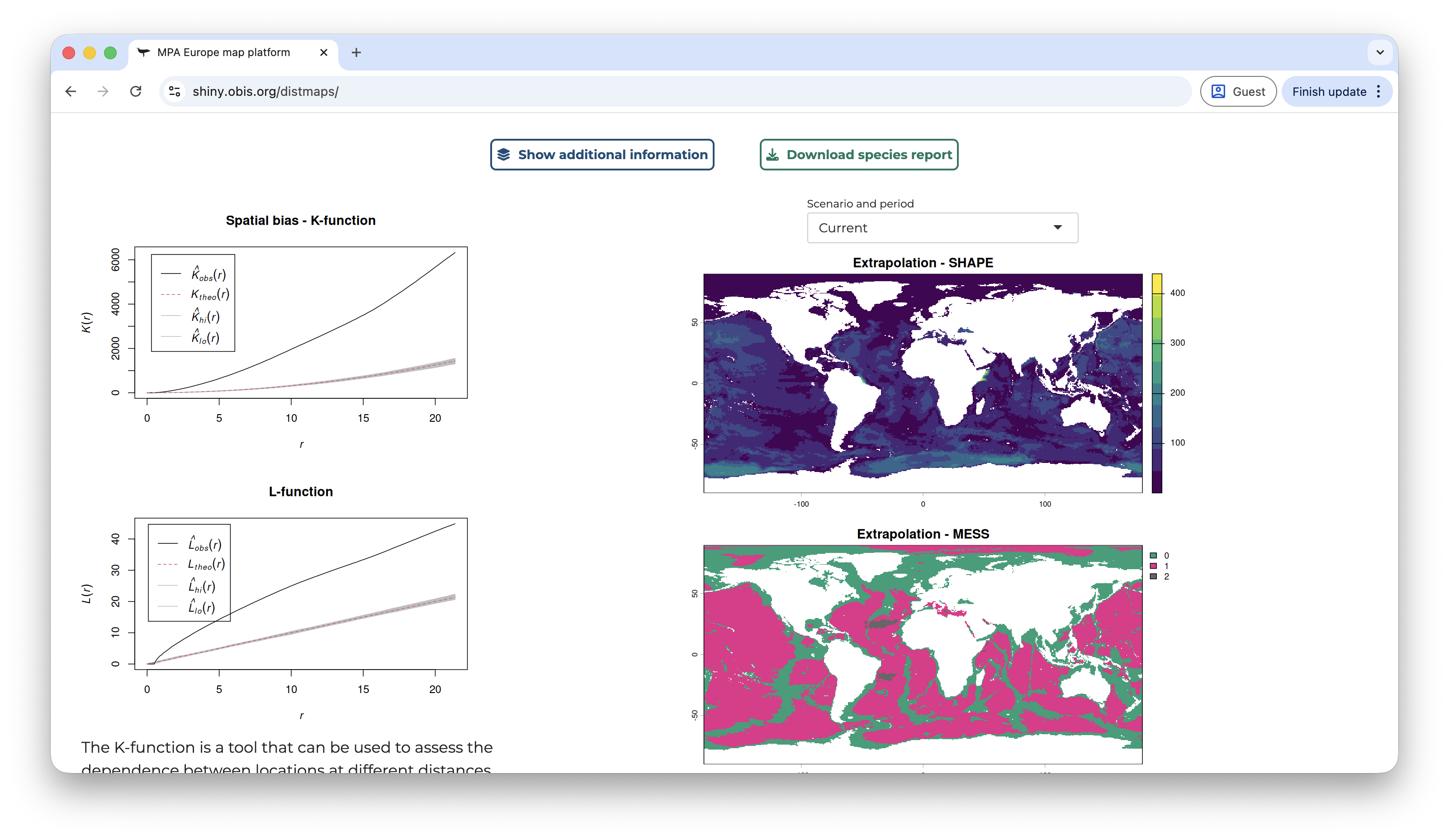
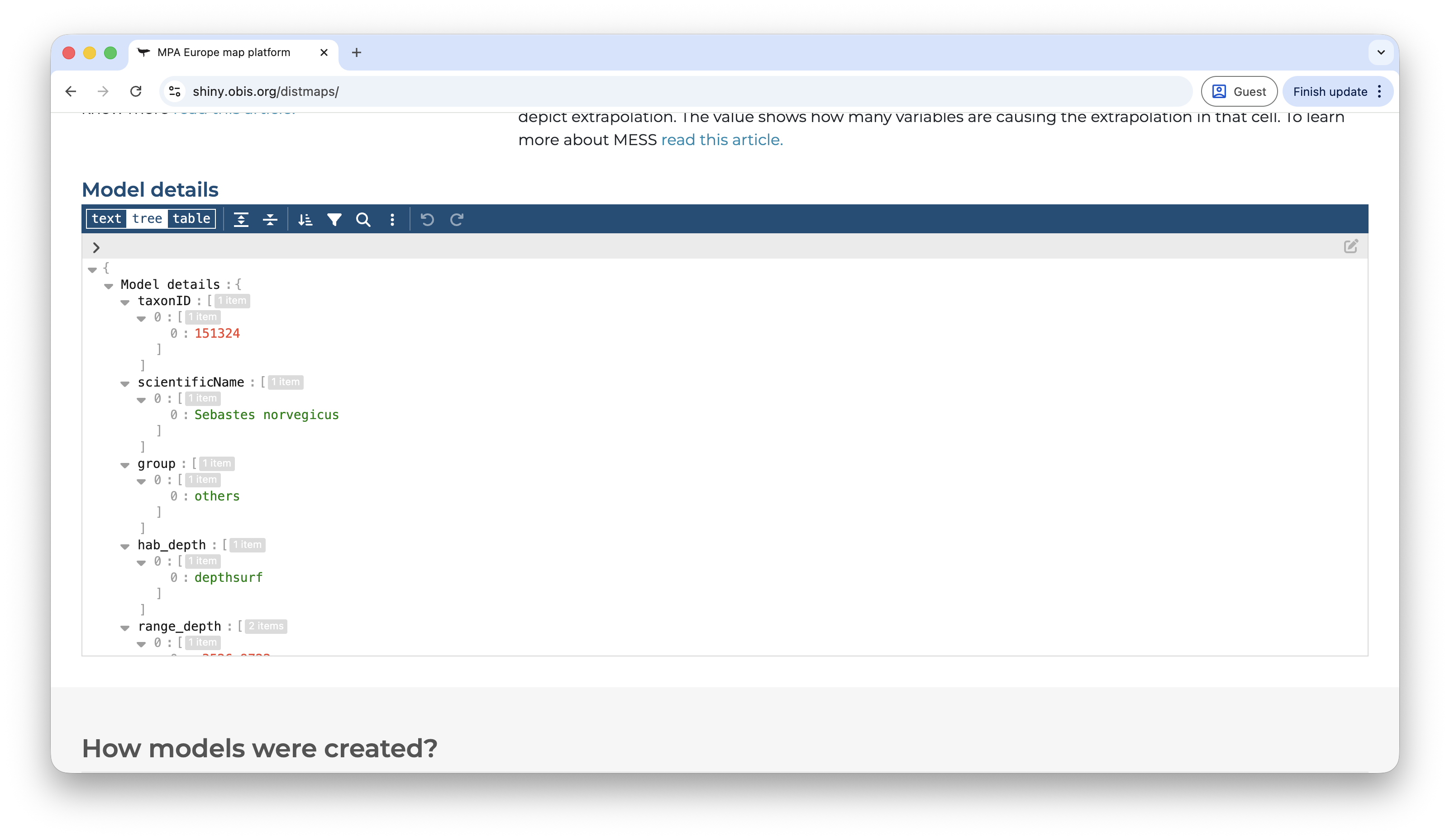
Below this section, there are two buttons to either download a species report or to show additional information. Under additional information the user has access to metrics of spatial bias in the data, extrapolation measures, and full model details.
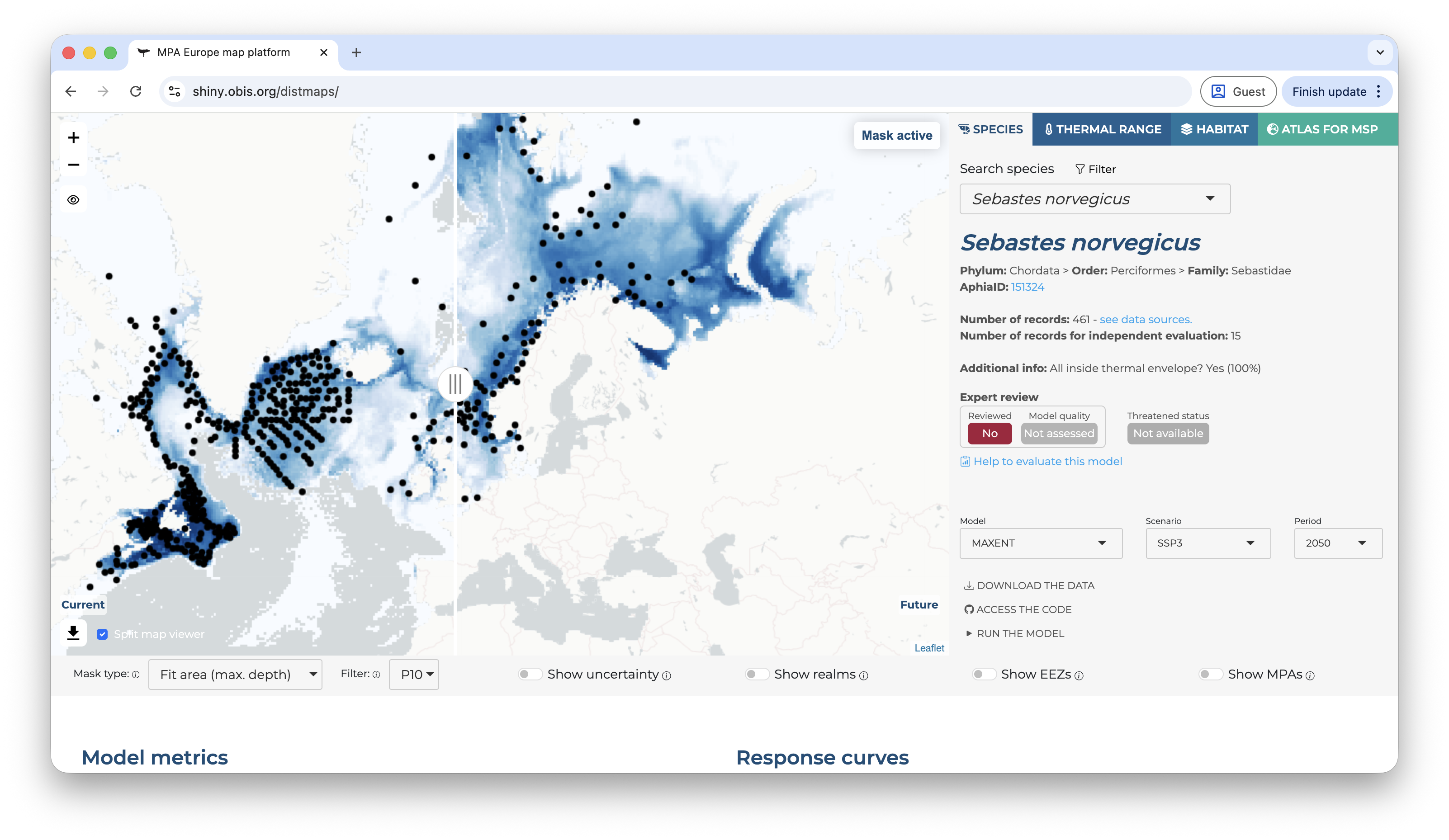
Back on the right panel, once you select a scenario different than the current, a control of the time period will also appear. At the same time, on the map panel, on the bottom-left corner you will find a button to split the viewer, showing at the same time the current and future prediction. This is useful to compare how the future prediction relates to the prediction of the current range of the species.
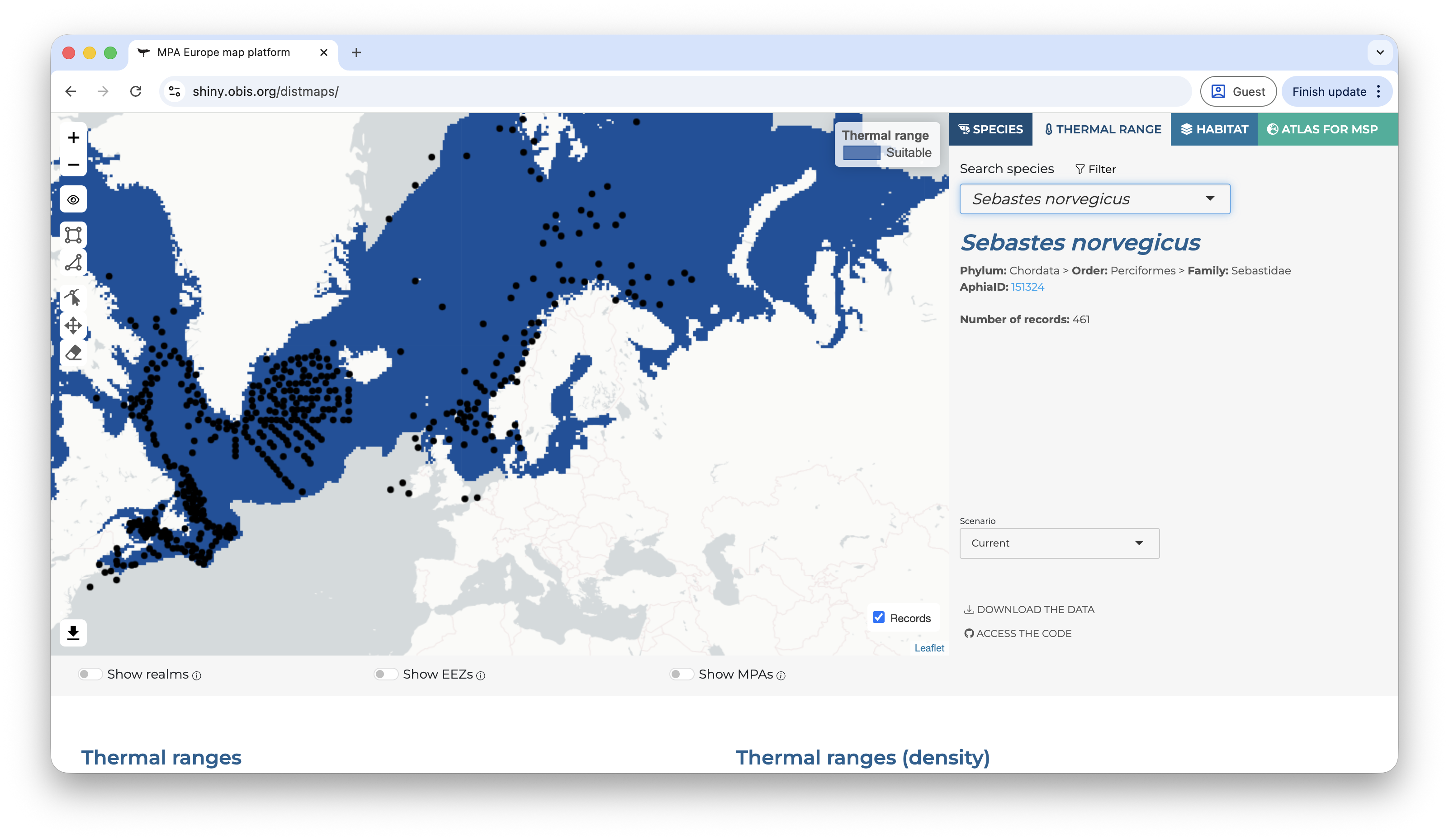
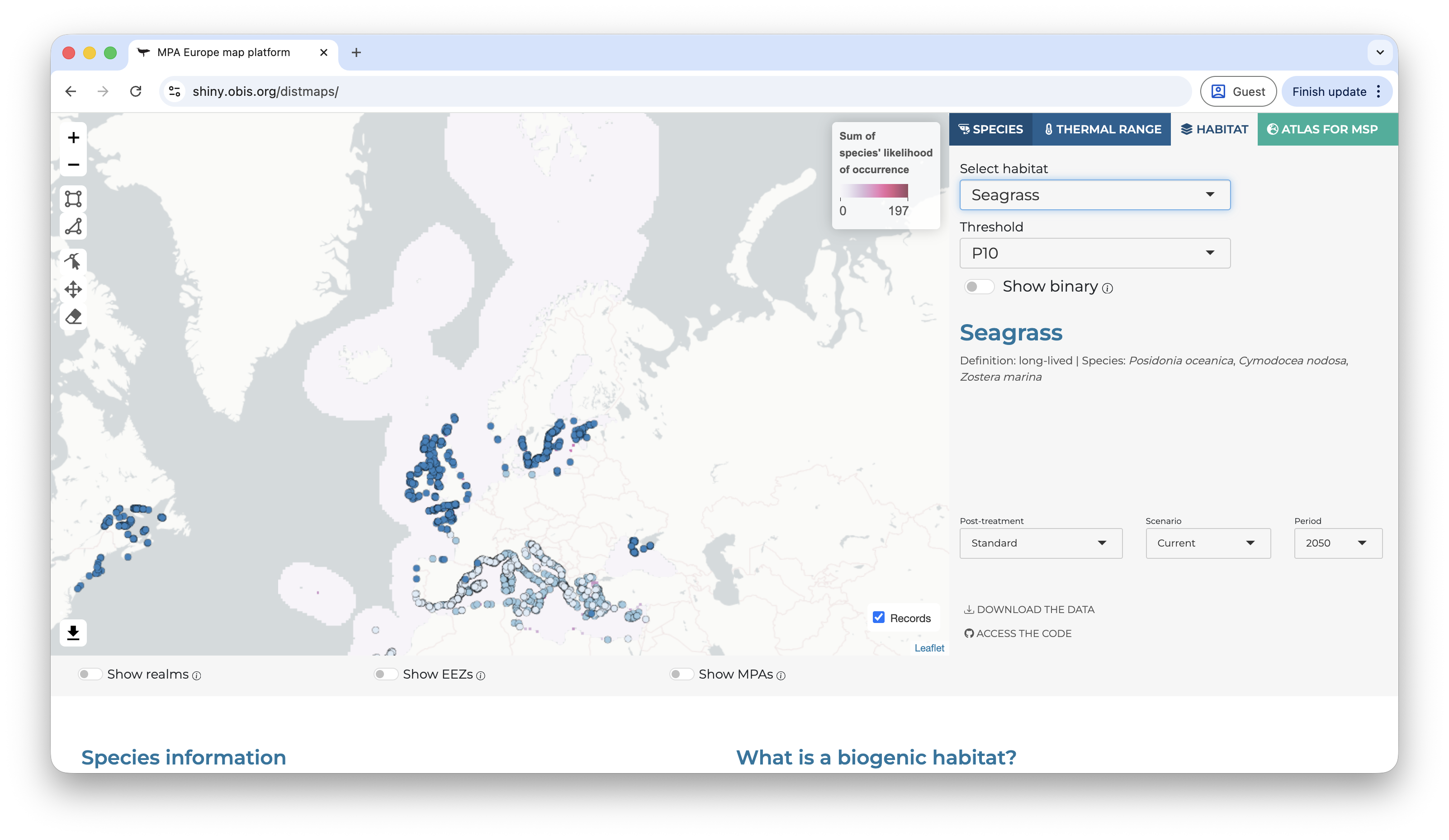
The user can also explore the additional tabs, like maps of the thermal range of the species (derived from the occurrence records) and the habitat maps (SSDMs).
6.2 Analyzing locally
All predictions and the raw (quality-controlled) data, as well as additional files (e.g. model metrics) are available through an AWS S3 bucket.
To explore the files available, go to https://obis-maps.s3.amazonaws.com/index.html and select sdm.
6.2.1 Using a file without dowloading
In many cases you can directly access the files from the S3 bucket. For example, on R, using the terra package, you can directly open the cloud-optimized GeoTIFF by providing the http address of the file:
If you want to download only a specific file, you can use the explorer to locate the file and then click on it to download.
Download complete species folders
To download a specific folder, the best way is to use the aws CLI program (see here). For example, if we want to download data for the species Echinus esculentus, we need only its AphiaID, which you can find on WoRMS. In this case the AphiaID is 124287 Then, from the command line we can do:
├── index.html
├── sdm                    : All distribution modelling results for the MPA Europe project
    ├── species                : Species Distribution Modelling results
    │   ├── ...
    │   └── taxonid=[AphiaID]  : Data for each species
    │
    ├── habitat                : Habitat Distribution Modelling results
    ├── diversity              : Diversity maps and analyses
    ├── source                 : Additional data necessary for running the models, not possible to store on GitHub
    └── stac                   : STAC catalogue for the files
And thus for accessing any species folder you just need:
s3://obis-maps/sdm/species/taxonid= + the AphiaID of the species
It is also possible to do this operation through R using the aws.s3 package:
install.packages("aws.s3")# Sync the contents of an S3 bucket subfolder to your local folders3sync(bucket ="obis-maps", prefix ="sdm/species/taxonid=124287", # Subfolder in the bucketsave_to ="./your-folder", # Local folderregion ="", # Region can be left empty for public bucketsuse_https =TRUE# This is equivalent to "--no-sign-request")
Warning
You can also sync (download) the full results folder using the AWS CLI with the following command:
However, this will download a few terabytes of data. So, we definitely do not recommend this approach.
Tip
See the section Section 6.3.3 to understand how you can use the STAC catalogue to organize your downloads and/or data access in a more efficient way.
6.2.3 Data structure
Outputs from WP3 (Biodiversity modelling) always follow the same standard structure. File names will always contain at least two components:
taxonid=[AphiaID]: identify the taxon model=[Model run acronym]: identify the modelling exercise
Additional information also follow a similar syntax (inspired on the hive format) and is identified by “[the parameter]=[the value]”. For example, a prediction file for a species will look like this:
method is the algorithm used for the model and scen the scenario and period of the prediction. In this case _cog simply indicates that the output is a cloud-optimized GeoTIFF.
A species folder have the following structure:
├── figures                    : Plots for quick exploration of results
├── metrics                    : All metrics and additional information (e.g. CV metrics, response curves, etc.)
├── models                     : RDS files containing the fitted models, ready for predicting in new data
├── predictions                : The TIF files with predictions
│
├── ..._what=fitocc.parquet    : Occurrence points used to fit the model
└── ..._what=log.json          : The log file containing all model fit details
We will see the folder metrics and predictions in more details, but first it is essential to understand the file ..what=log.json.
6.2.3.1 Understanding the log file
The log file contains all details about the model fitting, including best parameters of model tuning. It is rich document that enable easier reproduction of the results obtained. Here is a sample log file for the species with AphiaID 13185 (taxonid=135185_model=mpaeu_what=log.json):
You can open this file in any text editor in your computer, or through R using for example the jsonlite::read_json(). The package obissdm contains the function view_log to help visualize those files.
Each parameter is explained below:
6.2.3.2 The metrics folder
This is an example of the content of a metrics folder:
..._what=fullmetrics.parquet": metrics for the full model
..._what=respcurves.parquet": partial response curves for each variable
..._what=thresholds.parquet: thresholds that can be used to
..._what=biasmetrics.rds: an RDS file with metrics of data spatial bias
..._what=posteval_hyperniche.parquet: post-evaluation metrics for the hyperniche model
..._what=thermmetrics.json: thermal metrics
Note
Most files are in parquet format, which is a very efficient storage format. The easiest way to work with this type of data is through R, using the arrow package: arrow::open_dataset("parquet-file.parquet"). This will open a data.frame (tibble) that you can use as usual. If you don’t know R or any other programming language, then you can use an extension (on Google Drive, for example).
Two files are specially important: the cvmetrics which contain the metrics to assess the model predictive capacity, and thresholds which contains the values necessary for converting the predictions into binary format (if necessary). See the section “Analyzing the data” to understand more about the content of these files.
6.2.3.3 The predictions folder
This is an example of the content of a predictions folder:
Even more files available, but again many are just the same for different methods. The unique types of files are:
predictions: spatial predictions of models (following the pattern ..._method=[name of algorithm]_scen=[scenario and if applicable period]_cog.tif)
bootstrap: uncertainty in the models assessed as bootstrap. May not be available to all algorithms. Files follow the same pattern as the predictions, with what=boot added.
mask: the file named _what=mask_cog.tif contains the mask to limit predictions to specific areas (e.g. the native areas)
MESS map (uncertainty): the file _what=mess_cog.tif contains the MESS analysis, which measures extrapolation
SHAPE map (uncertainty): as MESS, the file _what=shape_cog.tif contains the SHAPE analysis which measures extrapolation
Thermal envelopes: the only file that is not a GeoTIFF is the _what=thermenvelope.parquet. This is a GeoParquet which contains the shapefiles of thermal envelopes for the species in different scenarios.
6.3 Processing data
You can analyze the SDM data in the tool you prefer - either through a programming language like R or Python, or using GIS programs like QGIS and ArcGIS. Here we will provide codes examples in R, the language used to produce the models, and also some examples in QGIS.
Note that for working in GIS programs, for some applications you will need to convert the Parquet files to CSV. There are multiple ways of doing that: you can use the R arrow package or Python pandas library. If you downloaded your data through the maps platform, then files are already in .csv format.
class       : SpatRaster
size        : 3600, 7200, 1  (nrow, ncol, nlyr)
resolution  : 0.05, 0.05  (x, y)
extent      : -180, 180, -90, 90  (xmin, xmax, ymin, ymax)
coord. ref. : lon/lat WGS 84 (EPSG:4326)
source      : taxonid=135185_model=mpaeu_method=maxent_scen=current_cog.tif
name        : current
min value   :       0
max value   :      98
plot(current)
All predictions folders always include a mask file. Let’s also open this file. The maskfile is a multiband raster, with each band being a different mask. We plot here the “fit_region_max_depth” mask.
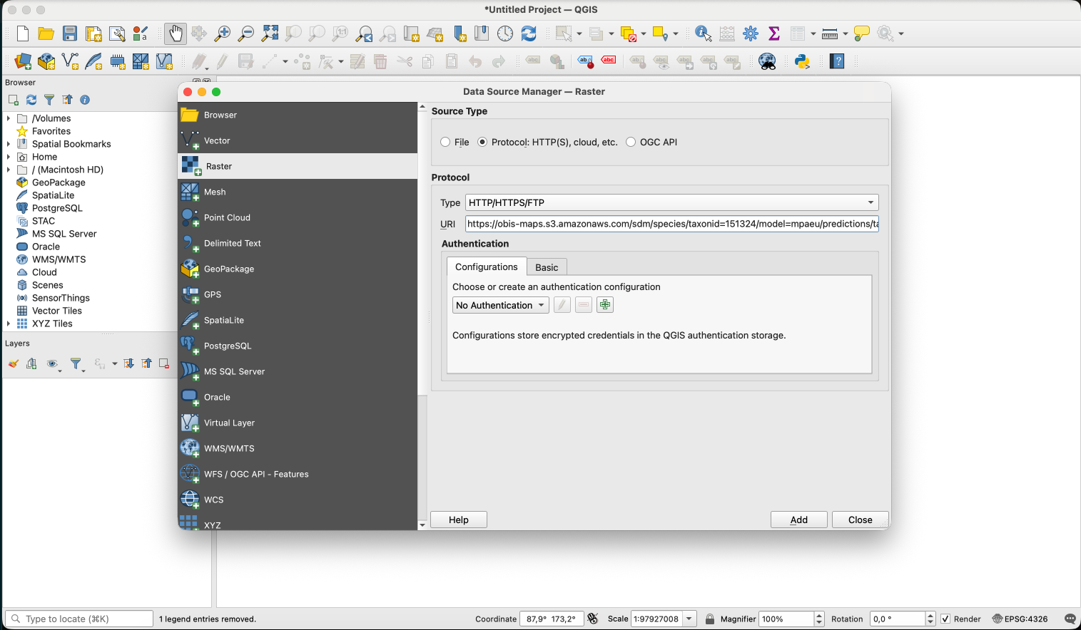
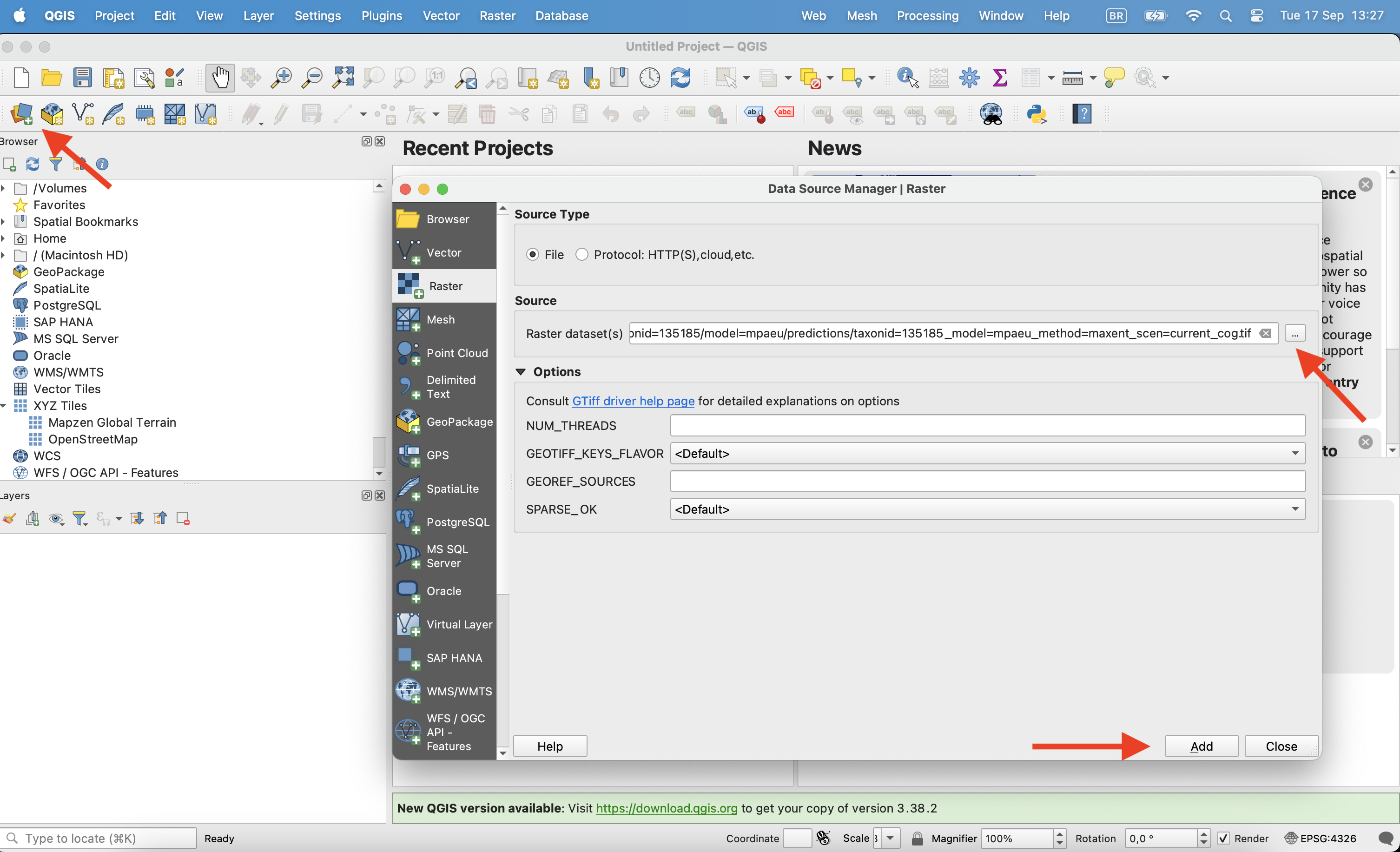
Open the file on QGIS clicking on the Open data source manager on the corner. Chose the raster file you want to open and click ok.
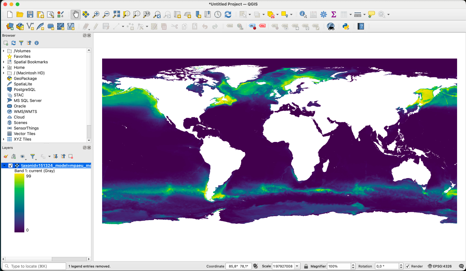
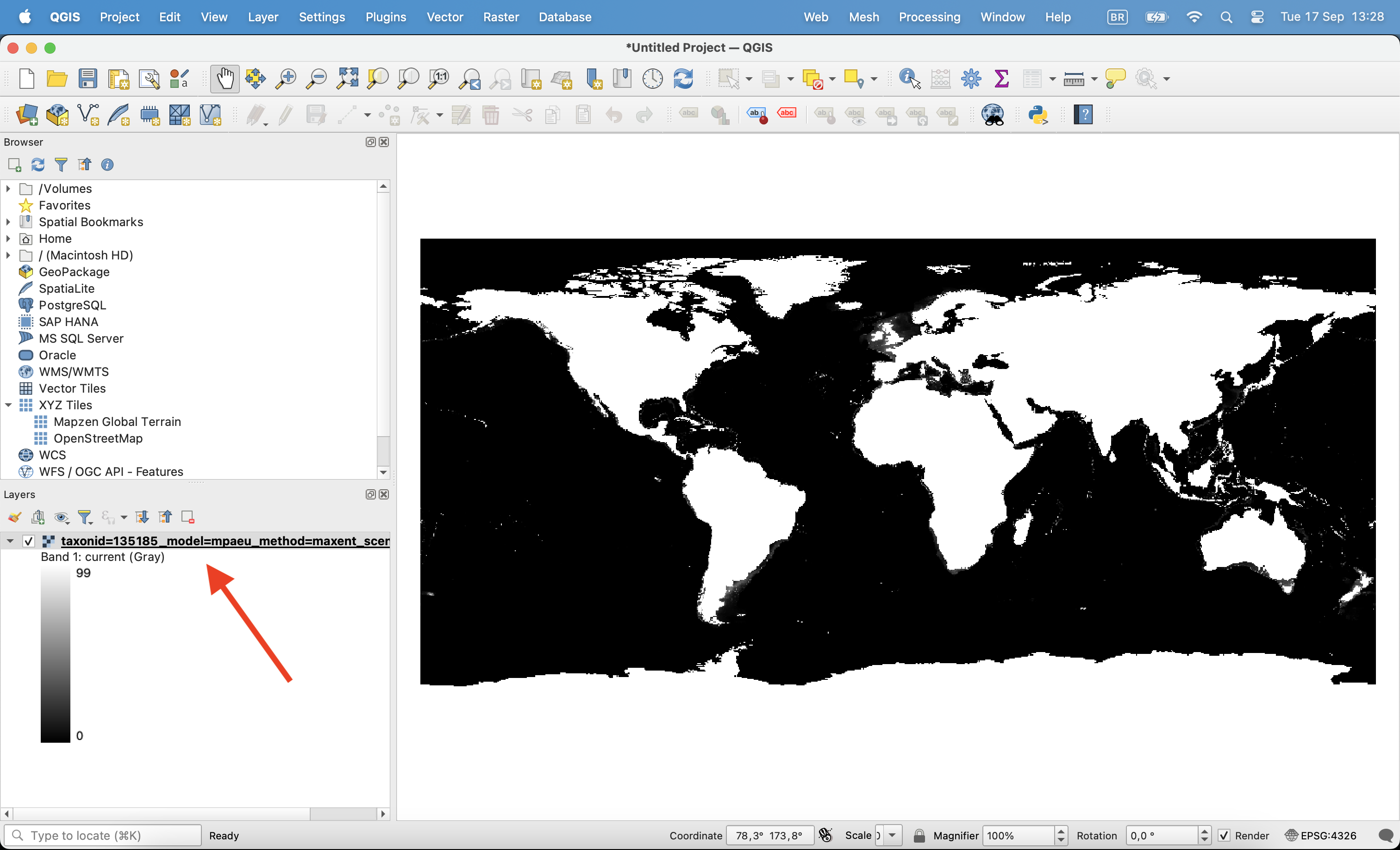
Once opened, click with the right button on the layer and click in properties.
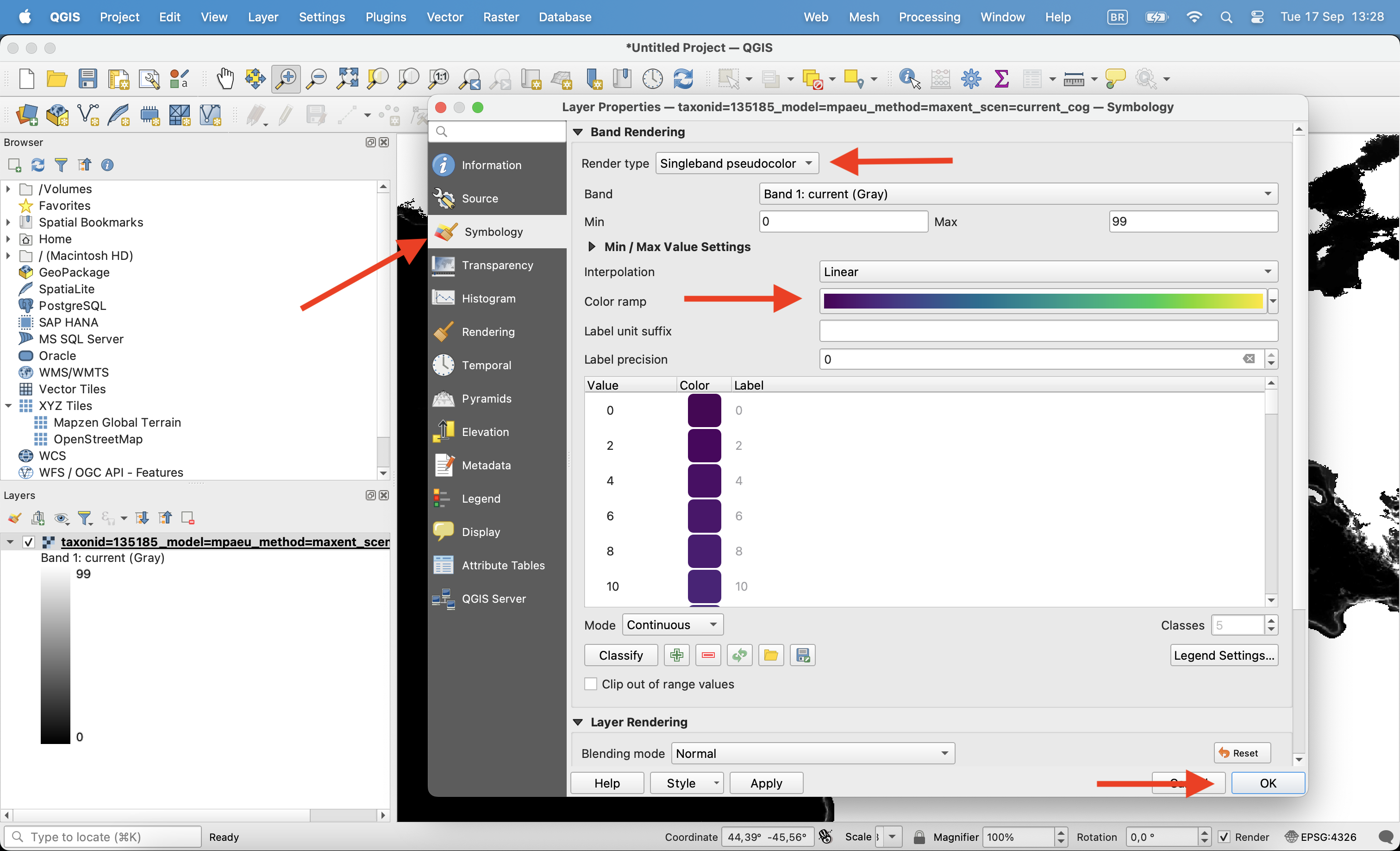
Then, on the Symbology tab change render type to ‘Singleband pseudocolor’, chose the color ramp and click ok.
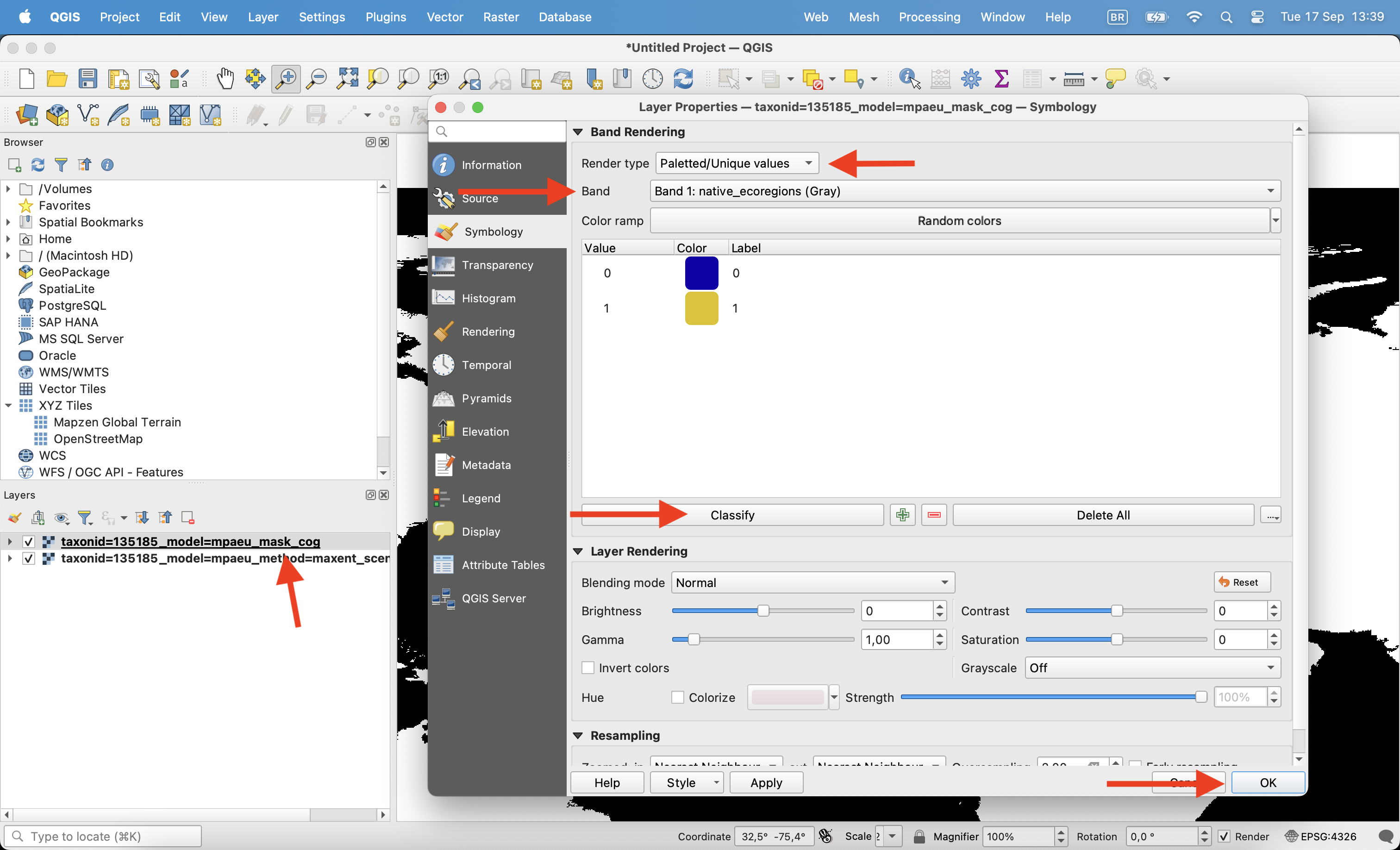
All predictions folders always include a mask file. Let’s also open this file. The maskfile is a multiband raster, with each band being a different mask. You can click with the right button, enter in properties and chose to visualize only one of the bands. Use the “Paletted/Unique values” option to color this layer (0/1).
6.3.2 Applying masks and converting to binary
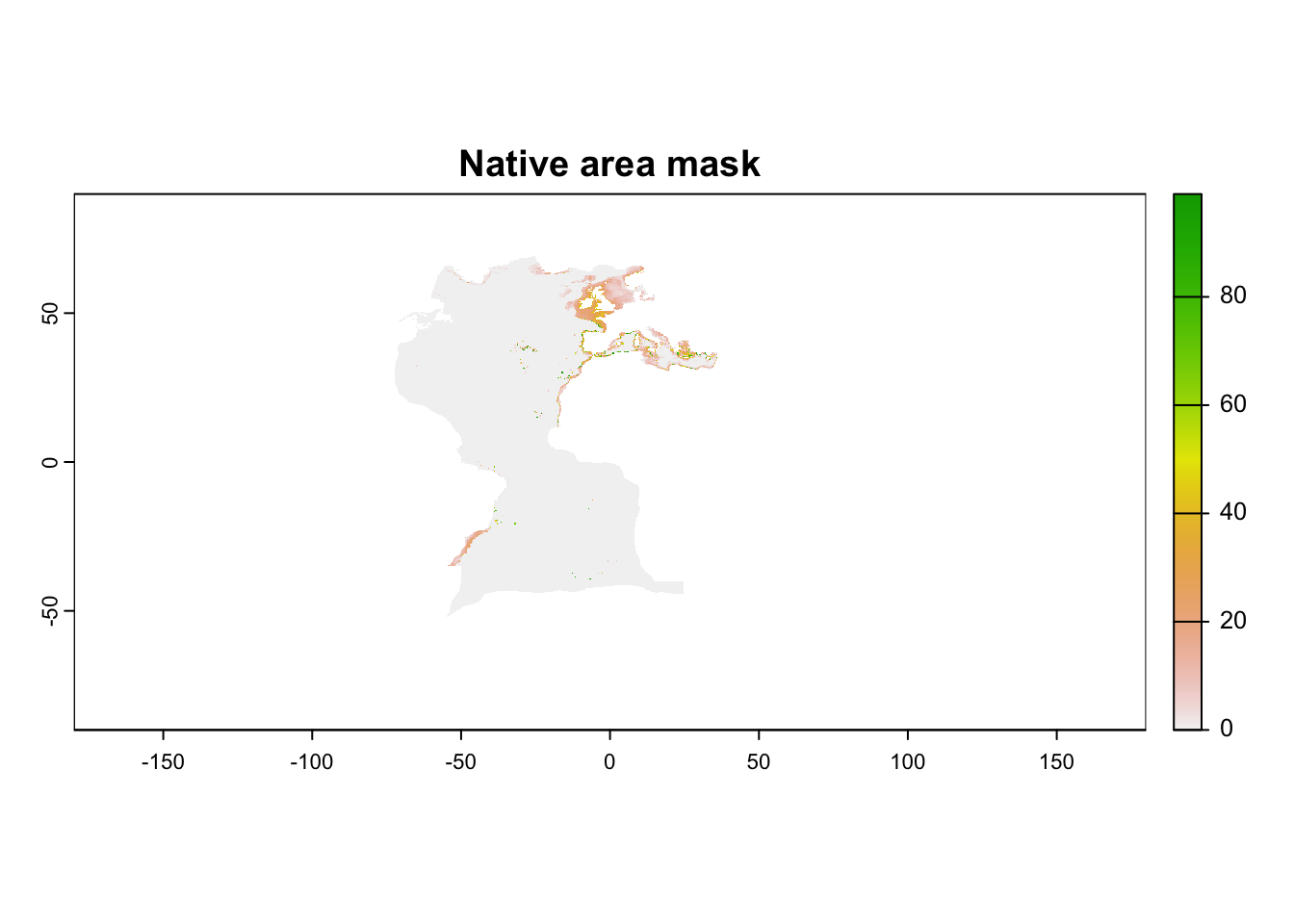
Predictions show the relative suitability of a place, in terms of its environmental conditions. However, predictions are made to the whole globe, including areas which may not be reachable by the species. Thus, it is always advisable to mask the predictions by one of the masks provided (or you can create one based on your hypothesis). In this case, we will use the realms in which the species occurs today (what we assume to be the “native area” of the species).
On R, the first step is to set the 0 values (negative mask) as the NA values, which is necessary by the function. Then we apply the target mask to our prediction:
NAflag(mask_file) <-0# terra function to set 0 as the NA flagcurrent <-mask(current, mask_file$native_ecoregions)plot(current, main ="Native area mask")
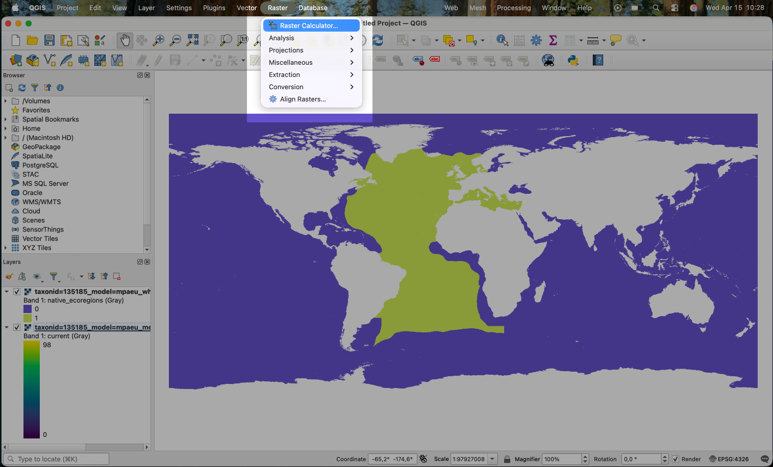
On QGIS we can apply the mask by using the Raster Calculator. Go to Raster > Raster Calculator.
Since the mask is a 0/1 file, this is a very simple operation: we will simply multiply the model prediction with the mask. You can select the raster bands on the menu. Note that the band names are not exhibited on this menu. You can first explore the band names by right clicking on the layer and selecting “Properties”. Under the “Information” tab you will find the bands list with its names.
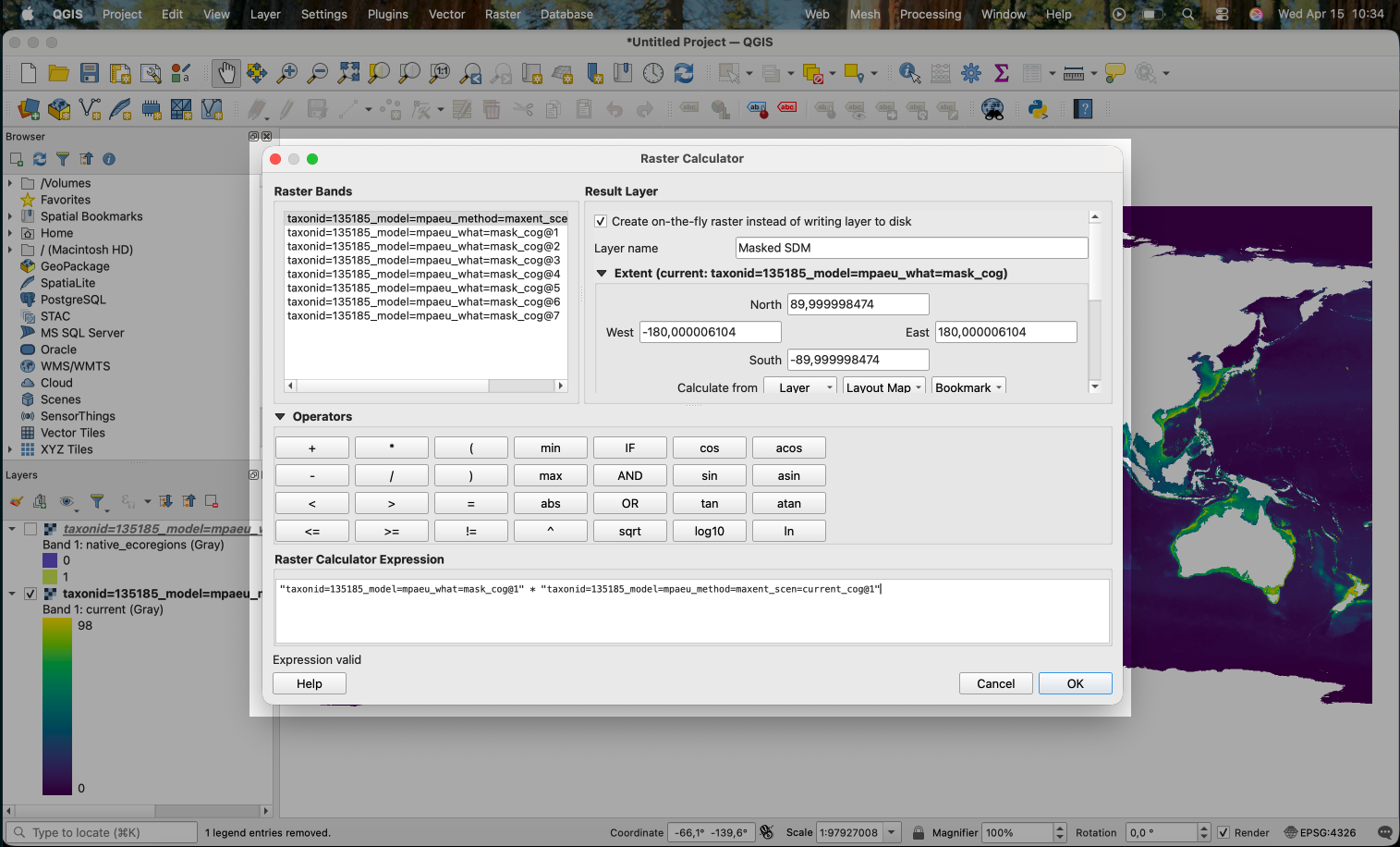
We use the following expression in the calculator:
That is, we are multiplying the first band of the mask (the @1 in the end of the name) with the first (unique) band of the prediction. Areas in the prediction where the mask is 0 will become 0 in the result.
Note that we selected “Create on-the-fly raster instead of writing layer to disk” to create an in-memory result layer (you can also directly save the result by not chosing this option).
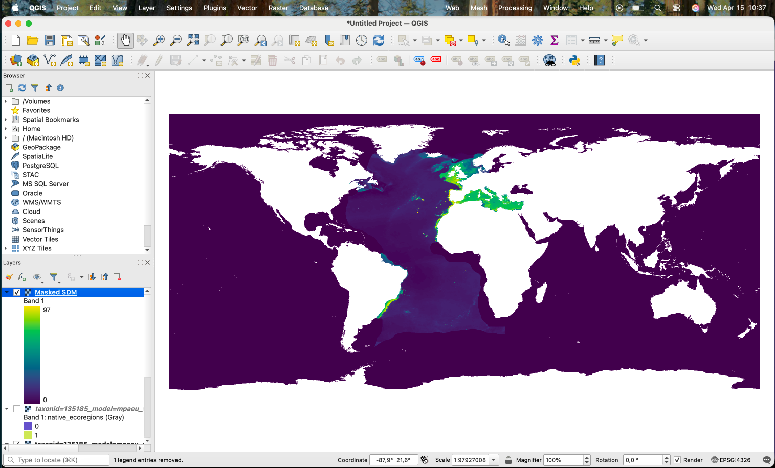
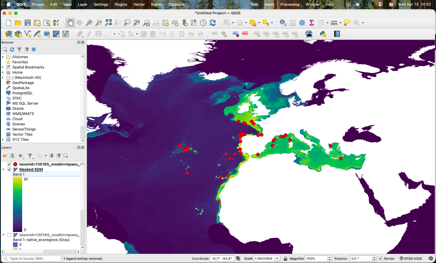
The result is now available in the main panel:
Now that we masked the prediction, we may want to limit it to only areas that are more likely to have the species according to a certain threshold. Ideally, you should always work with continuous predictions, but in some cases a binary map (presence/absence of species) may be desirable. We will also load the occurrence data.
On R, we start by loading the occurrence data and the table with thresholds. Here we will apply the P10 threshold, which removes all values lower than the 10th percentile of values in the occurrence records.
library(arrow)records <-read_parquet("files/results/taxonid=135185/model=mpaeu/taxonid=135185_model=mpaeu_what=fitocc.parquet")thresholds <-read_parquet("files/results/taxonid=135185/model=mpaeu/metrics/taxonid=135185_model=mpaeu_what=thresholds.parquet")p10 <- thresholds$p10[thresholds$model =="maxent"]p10 <- p10 *100# to put on the same scale, see note below
Important
The thresholds are expressed on the scale 0-1 (with decimals), the same as the original predictions. However, to improve the storage efficiency, all predictions are first multiplied by 100, and then saved as integers. Thus, before applying the threshold you should multiply it by 100 (or divide the prediction by 100, if you prefer it in the original scale).
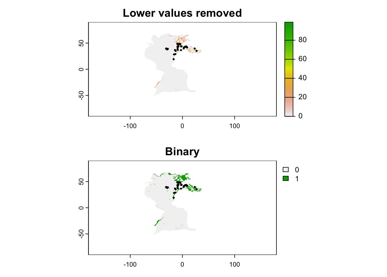
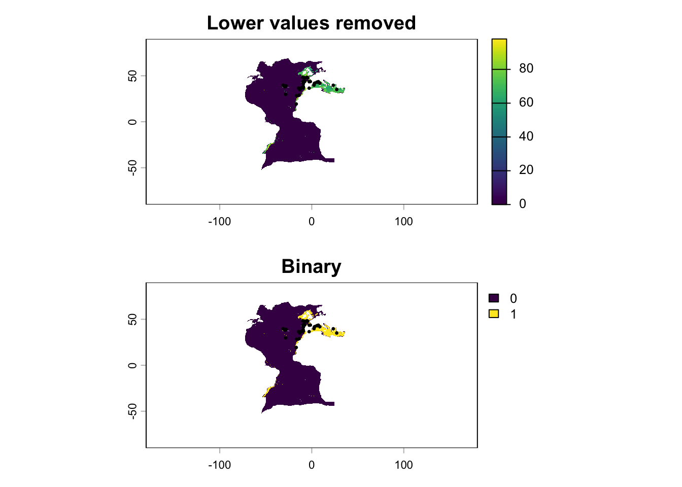
And then we apply the threshold to the map. We will do the two modes: the first simply remove areas below the threshold and the second actually converts in binary format.
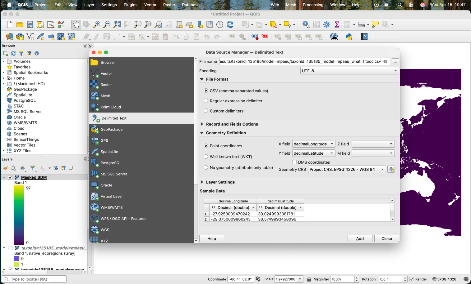
On QGIS, we start by adding the occurrence records. We use a CSV file (we first converted the Parquet file to CSV on R).
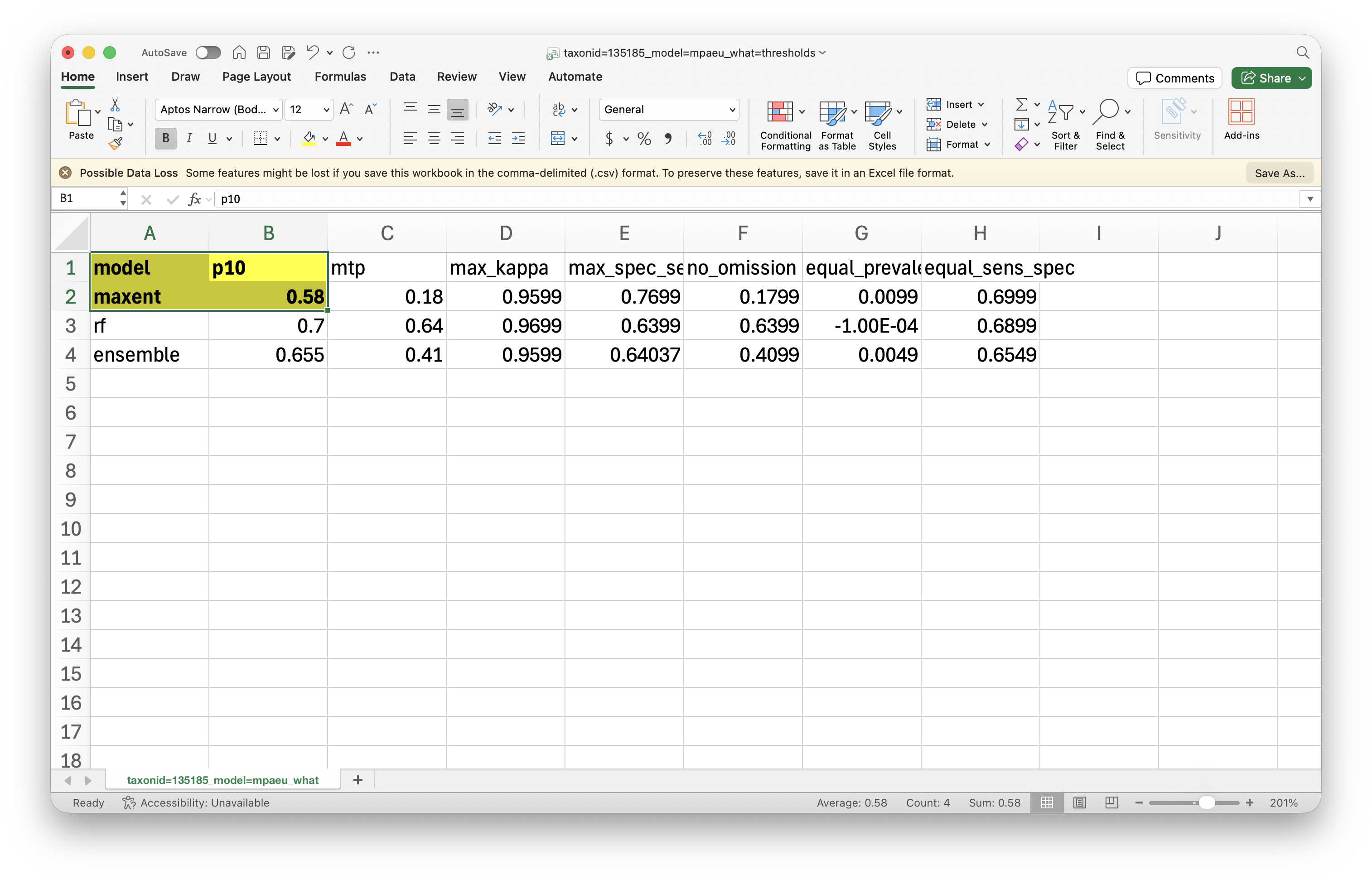
To apply the thrshold, we open the CSV file and look at the column with the corresponding threshold and the line for the target model. Here we will apply the P10 threshold, which removes all values lower than the 10th percentile of values in the occurrence records.
Important
The thresholds are expressed on the scale 0-1 (with decimals), the same as the original predictions. However, to improve the storage efficiency, all predictions are first multiplied by 100, and then saved as integers. Thus, before applying the threshold you should multiply it by 100 (or divide the prediction by 100, if you prefer it in the original scale).
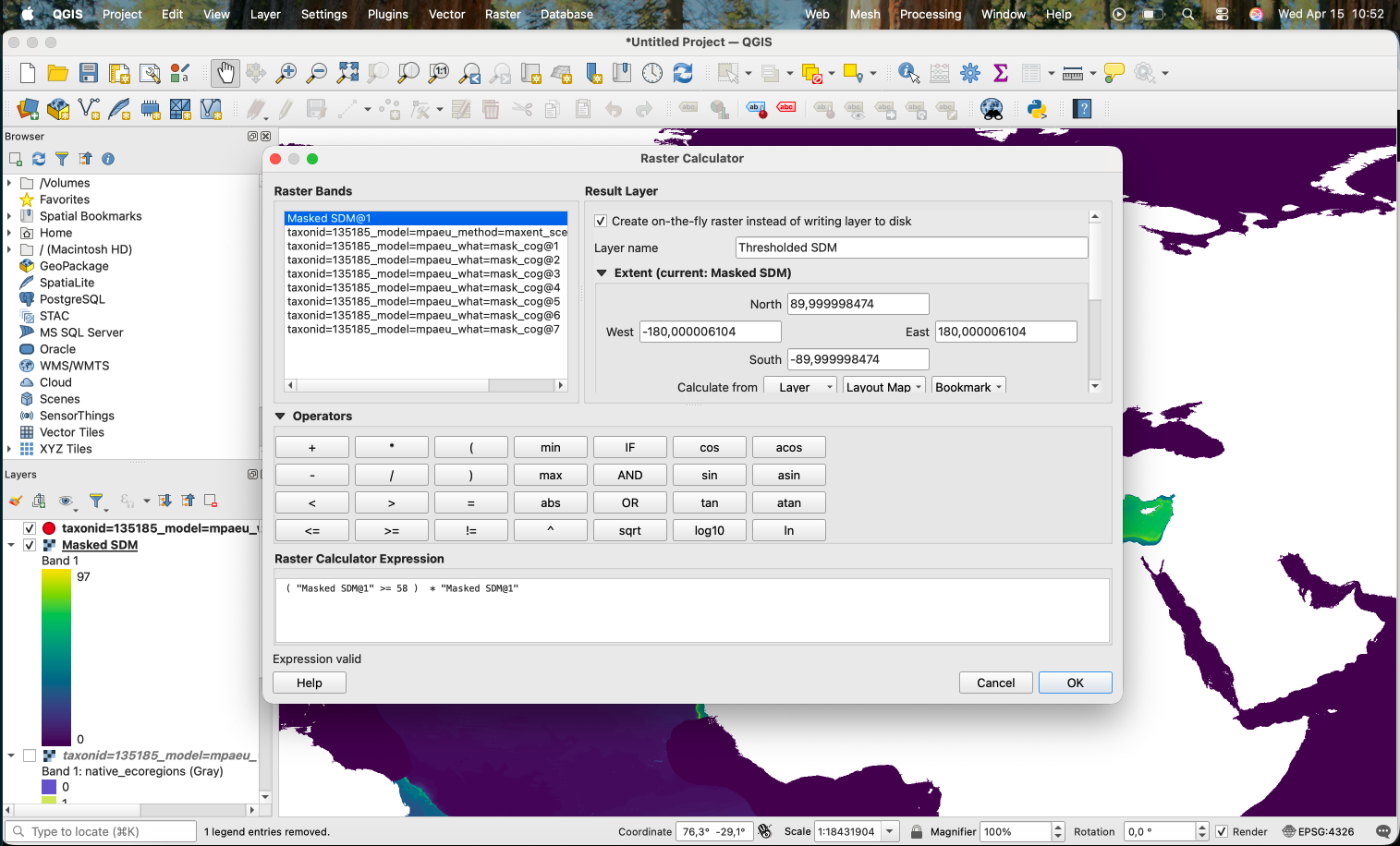
We will once more use the Raster Calculator, which you access from Raster > Raster Calculator.
We need to get a “mask” of the areas where the values are higher or equal the threshold (in this case 0.58 * 100 = 58). This will produce a file with 0 and 1 (1 for the areas that are >= the threshold). We then multiply this by the original layer, what removes (turn into 0) the areas that are below the threshold. This is the expression we use:
( "Masked SDM@1" >= 58 ) * "Masked SDM@1"
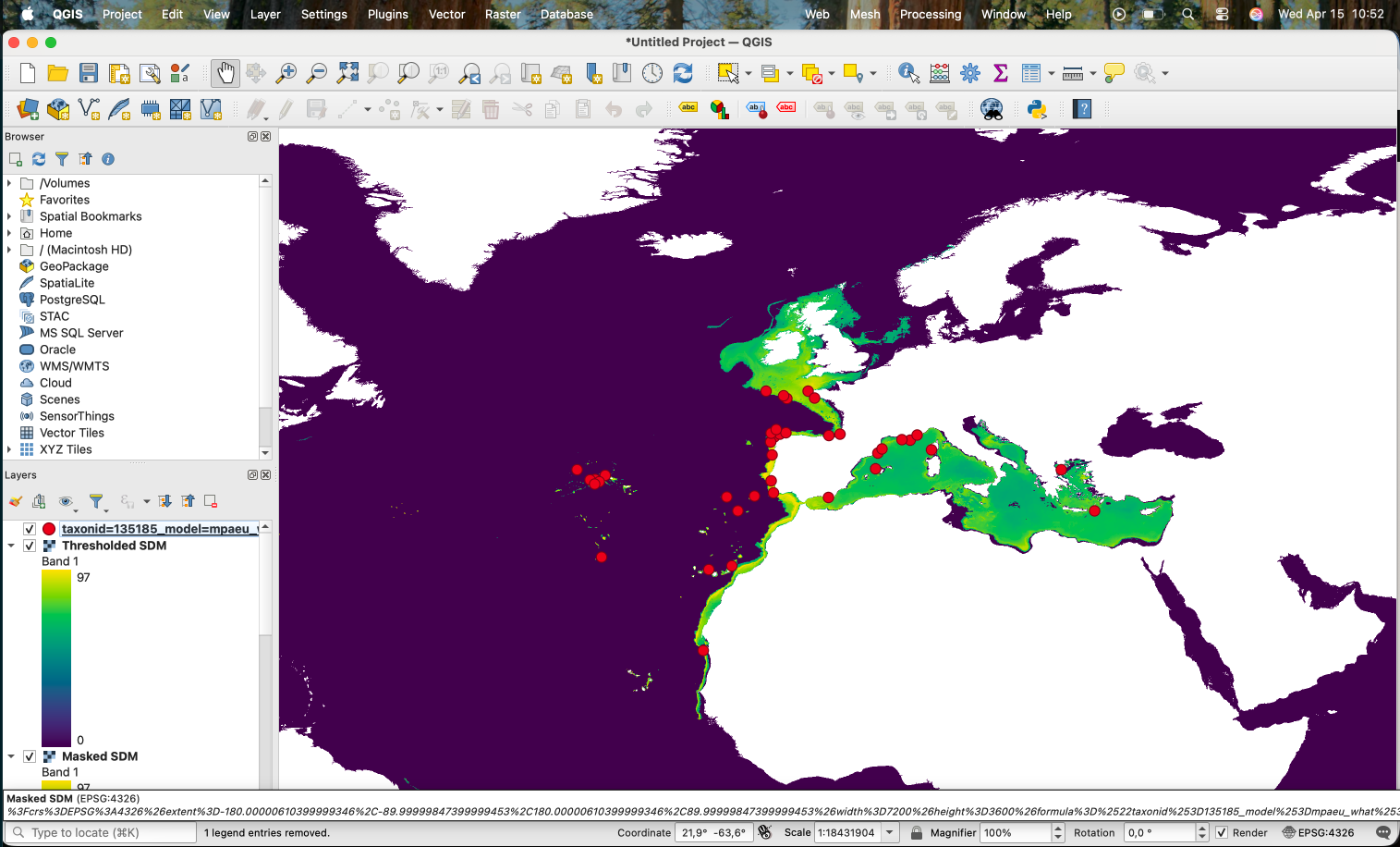
Which results in the areas with low suitability according to the threshold being removed:
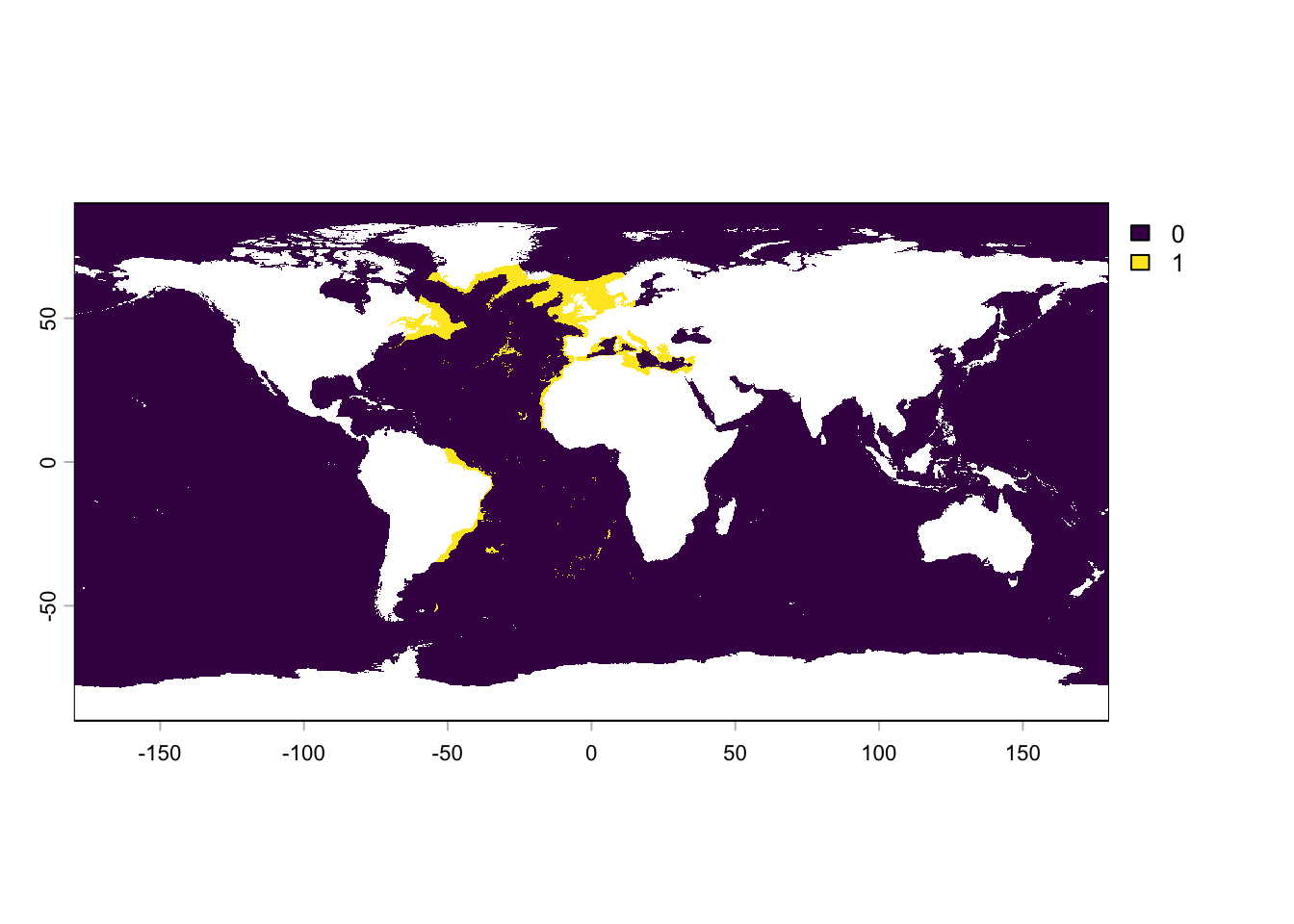
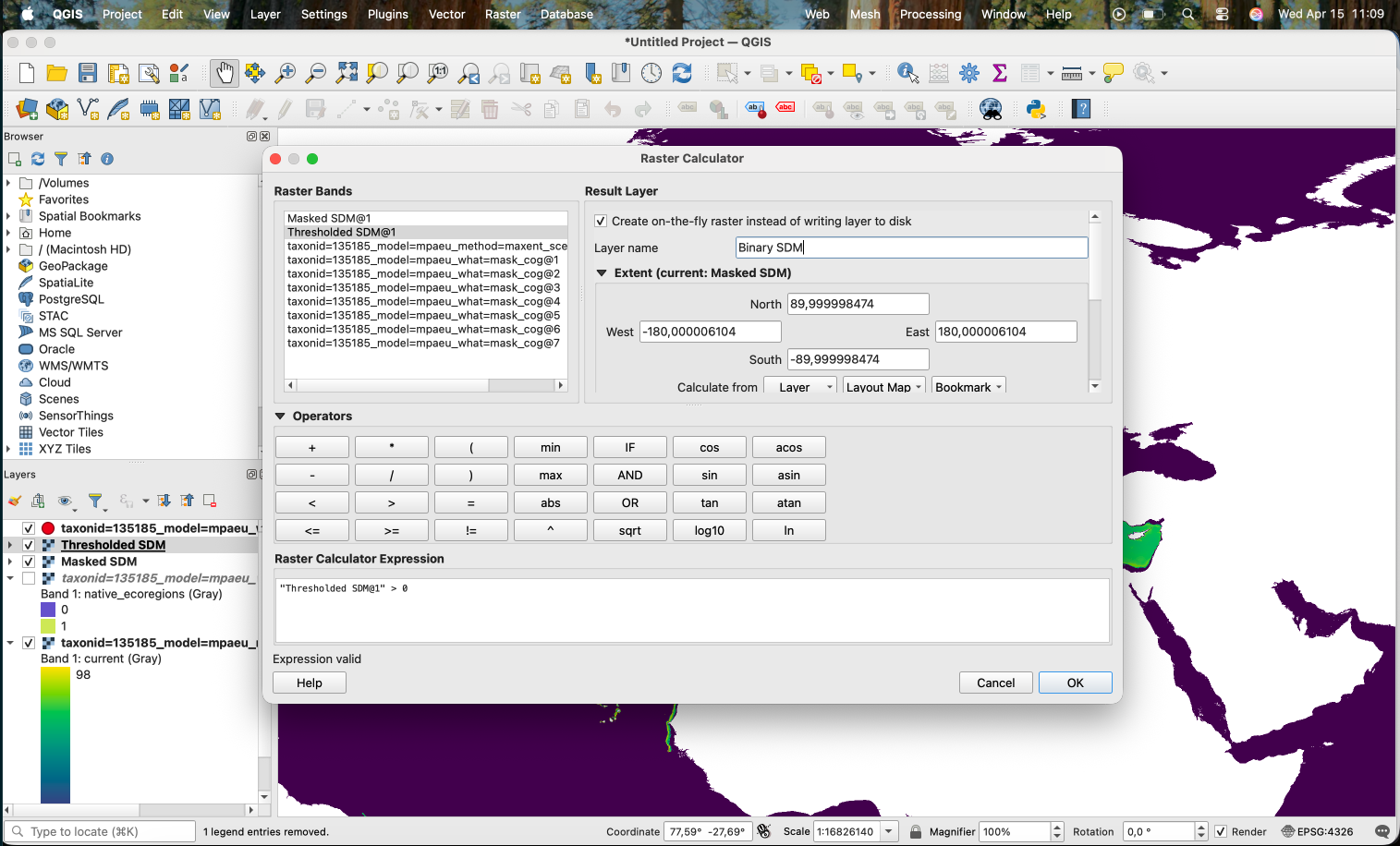
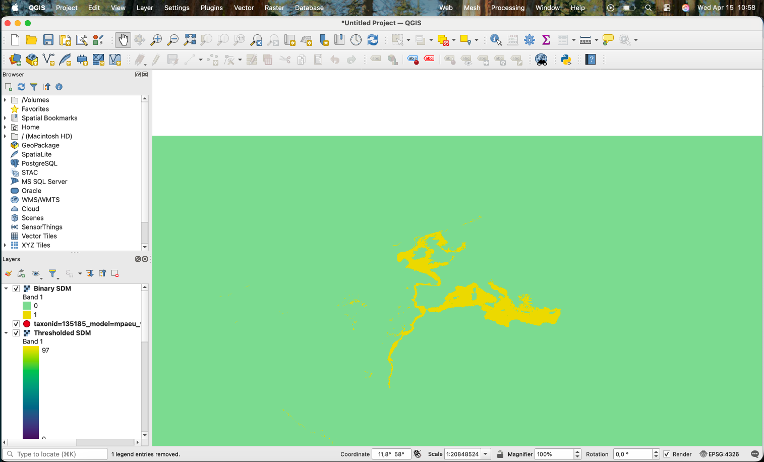
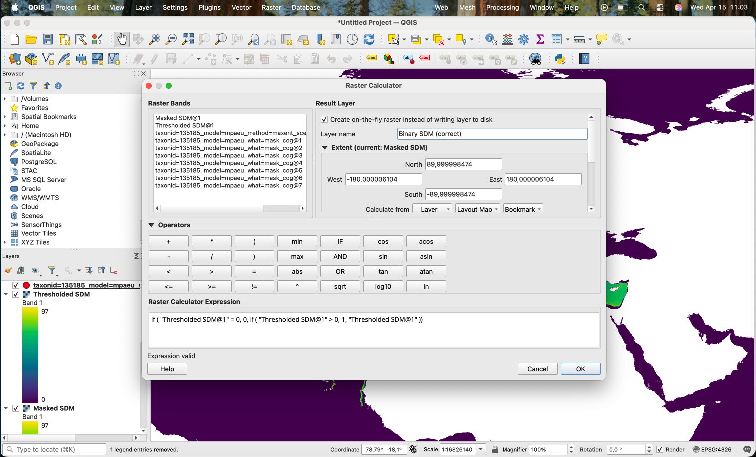
If we want to produce a binary version (0/1), we can use the Raster Calculator with the expression "Thresholded SDM@1" > 0:
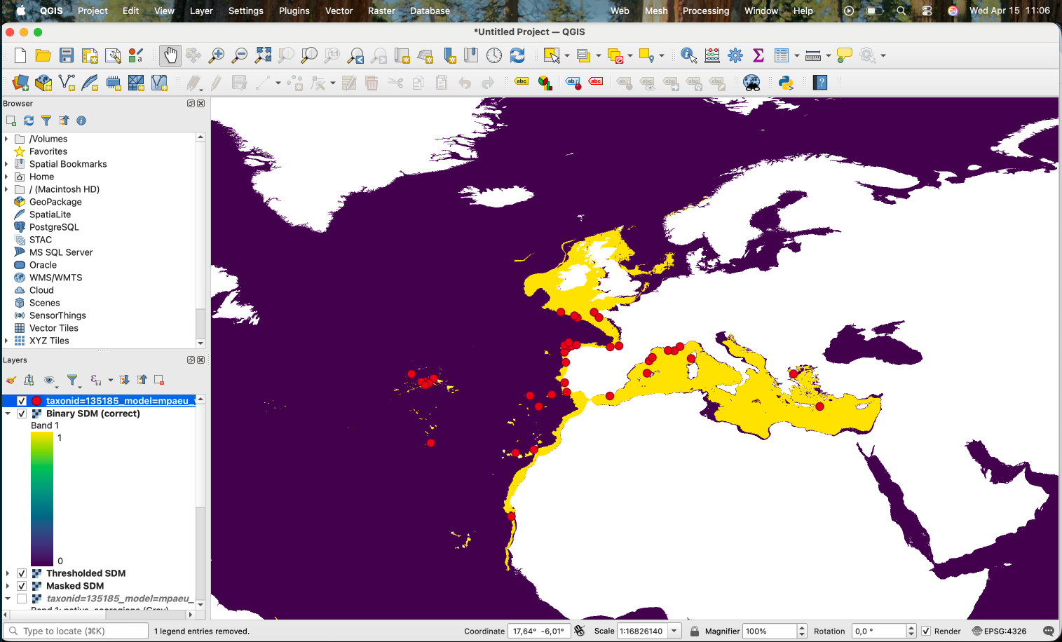
This works, producing the following:
However, as you can notice, the areas that were originally NA (i.e. the land) also become 0. An alternative is to use the following expression:
if ( "Thresholded SDM@1" = 0, 0, if ( "Thresholded SDM@1" > 0, 1, "Thresholded SDM@1" ))
Which will keep the original values when the value is neither 0 or 1.
6.3.3 The STAC catalogue
Since version 2, the MPA Europe SDMs are organized in a STAC catalogue which you can find on s3://obis-maps/sdm/stac. The easiest way to explore it is through this page.
Depending on your needs, it might be interesting to use the STAC catalogue to organize your downloads. For example, suppose you are interested in obtaining the SDM for all species, but you just want one model and the current scenario. Not all models are available to all species, so first you need to know which models are available.
We start by loading the STAC metadata file. You can sync the full STAC to a local folder, but in this case we are going to directly access just the JSON file for the species collection:
List of 9
 $ type           : chr "Feature"
 $ stac_version   : chr "1.1.0"
 $ stac_extensions: list()
 $ id             : chr "taxonid=1005391"
 $ geometry       : NULL
 $ properties     :List of 9
  ..$ taxonid       : int 1005391
  ..$ model         : chr "mpaeu"
  ..$ scientificName: chr "Hexaplex kuesterianus"
  ..$ group         : chr "others"
  ..$ hab_depth     : chr "depthmean"
  ..$ fit_bbox      :List of 4
  .. ..$ : num 48.2
  .. ..$ : num 17
  .. ..$ : num 58.9
  .. ..$ : num 29.2
  ..$ fit_n_points  : int 17
  ..$ methods       : chr "esm"
  ..$ datetime      : chr "2025-01-01T00:00:00Z"
 $ links          :List of 3
  ..$ :List of 3
  .. ..$ rel : chr "root"
  .. ..$ href: chr "../../../../catalog.json"
  .. ..$ type: chr "application/json"
  ..$ :List of 3
  .. ..$ rel : chr "collection"
  .. ..$ href: chr "../collection.json"
  .. ..$ type: chr "application/json"
In this case we are interested in the properties. The option methods contain the name of the methods that are available for this species.
sp_item$properties$methods
[1] "esm"
We can then read this information for all species and select one method. Suppose you have a preference for methods in this order:
Ensemble > Maxent > RandomForest > XGBoost > ESM
We would then use this code:
pref_order <-c("ensemble", "maxent", "rf", "xgboost", "esm")# We will do to only the first 10 to speed up hereitems_df <- items_df[1:10, ]items_df$scientificName <-NAitems_df$model <-NAfor (i inseq_len(nrow(items_df))) { sp_item <-read_json(paste0(base_add, items_df$href[i])) items_df$scientificName[i] <- sp_item$properties$scientificName items_df$model[i] <- pref_order[which.min(match(sp_item$properties$methods, pref_order))]}head(items_df)