A global gap analysis for the eDNA Expeditions reference databases

Reference databases

Reference database creation is documented at https://github.com/iobis/eDNA_trial_data, and reference databases were downloaded to reference_databases from the LifeWatch server using:

rsync -avrm --partial --progress --include='*/' --include='*pga_tax.tsv' --include='*pga_taxa.tsv' --include='*pga_taxon.tsv' --exclude='*' ubuntu@lfw-ds001-i035.i.lifewatch.dev:/home/ubuntu/data/databases/ ./reference_databases
rm -r ./reference_databases/silva*

Species lists

Use the ednagaps package to WoRMS aligned species lists by marker.

library(ednagaps)
library(dplyr)
library(DBI)
library(sf)
library(leaflet)
library(ggplot2)
library(glue)

reference_databases <- list(
  "12s_mimammal" = list(
    taxa = "~/Desktop/temp/reference_databases/12S/202311/12S_mammal_ncbi_1_50000_pcr_pga_taxa.tsv"
  ),
  "12s_mifish" = list(
    taxa = "~/Desktop/temp/reference_databases/12S/202311/12S_mito_ncbi_1_50000_mifish_pcr_pga_taxa.tsv"
  ),
  "12s_teleo" = list(
    taxa = "~/Desktop/temp/reference_databases/12S/202311/12S_mito_ncbi_1_50000_teleo_pcr_pga_taxa.tsv"
  ),
  "coi" = list(
    taxa = "~/Desktop/temp/reference_databases/COI_ncbi/COI_ncbi_1_50000_pcr_pga_taxon.tsv"
  ),
  "16s" = list(
    taxa = "~/Desktop/temp/reference_databases/16S/202311/16S_ncbi_euk_1_50000_pga_taxa.tsv"
  )
)

generate_reference_species(reference_databases)

Then read the generated lists and add higher level taxonomic groups:

reference_species <- read_reference_species()
reference_species
#> # A tibble: 125,437 × 12
#>    marker       phylum   class    order family genus species isMarine isBrackish
#>    <chr>        <chr>    <chr>    <chr> <chr>  <chr> <chr>      <dbl>      <dbl>
#>  1 12s_mimammal Chordata Teleost… Perc… Serra… Cent… Centro…        1          0
#>  2 12s_mimammal Chordata NA       Test… Trion… Pelo… Pelodi…        0          0
#>  3 12s_mimammal Chordata Mammalia Arti… Bovid… Bos   Bos ta…       NA         NA
#>  4 12s_mimammal Chordata Mammalia Carn… Phoci… Mona… Monach…        1         NA
#>  5 12s_mimammal Chordata Mammalia Carn… Otari… Arct… Arctoc…        1         NA
#>  6 12s_mimammal Chordata Teleost… Cent… Kypho… Kyph… Kyphos…        1          0
#>  7 12s_mimammal Chordata Teleost… Cent… Kypho… Gire… Girell…        1          0
#>  8 12s_mimammal Chordata Teleost… Cypr… Cypri… Ache… Acheil…        0          1
#>  9 12s_mimammal Chordata Teleost… Cypr… Cypri… Ache… Acheil…        0          1
#> 10 12s_mimammal Chordata Teleost… Perc… Anarh… Anar… Anarrh…        1          0
#> # ℹ 125,427 more rows
#> # ℹ 3 more variables: isFreshwater <dbl>, isTerrestrial <dbl>, input <chr>

Occurrence data

H3 gridded occurrence data is read from a custom SQLite database:

con <- dbConnect(RSQLite::SQLite(), "~/Desktop/protectedseas/database.sqlite")

res <- dbSendQuery(con, "
  select phylum, class, \"order\", species, h3.h3_2 as h3 from occurrence
  left join species on species.scientificname = occurrence.species
  left join h3 on occurrence.h3 = h3.h3_7
  where phylum is not null
  group by phylum, class, \"order\", species, h3.h3_2
")
gridded_occurrences <- dbFetch(res) %>% 
  add_groups() %>%
  as_tibble()

dbClearResult(res)
dbDisconnect(con)

gridded_occurrences
#> # A tibble: 2,855,810 × 6
#>    phylum         class            order              species        h3    group
#>    <chr>          <chr>            <chr>              <chr>          <chr> <chr>
#>  1 Acanthocephala Eoacanthocephala Gyracanthocephala  Acanthogyrus … 8297… NA   
#>  2 Acanthocephala Eoacanthocephala Gyracanthocephala  Pallisentis (… 823d… NA   
#>  3 Acanthocephala Eoacanthocephala Neoechinorhynchida Atactorhynchu… 822b… NA   
#>  4 Acanthocephala Eoacanthocephala Neoechinorhynchida Atactorhynchu… 8244… NA   
#>  5 Acanthocephala Eoacanthocephala Neoechinorhynchida Atactorhynchu… 8244… NA   
#>  6 Acanthocephala Eoacanthocephala Neoechinorhynchida Atactorhynchu… 8244… NA   
#>  7 Acanthocephala Eoacanthocephala Neoechinorhynchida Atactorhynchu… 8244… NA   
#>  8 Acanthocephala Eoacanthocephala Neoechinorhynchida Atactorhynchu… 8244… NA   
#>  9 Acanthocephala Eoacanthocephala Neoechinorhynchida Atactorhynchu… 8244… NA   
#> 10 Acanthocephala Eoacanthocephala Neoechinorhynchida Atactorhynchu… 8245… NA   
#> # ℹ 2,855,800 more rows

Analysis

Completeness by group and marker

stats <- gridded_occurrences %>%
  group_by(group, species) %>%
  summarize() %>% 
  left_join(reference_species %>% select(marker, species), by = "species") %>%
  group_by(group) %>%
  mutate(
    group_species = n_distinct(species),
    group_species_in_reference = n_distinct(species[!is.na(marker)])
  ) %>%
  group_by(group, group_species, group_species_in_reference, marker) %>%
  summarize(
    group_marker_species = n_distinct(species)
  ) %>%
  ungroup() %>% 
  mutate(fraction = group_marker_species / group_species) %>%
  filter(!is.na(marker) & !is.na(group))

stats_combined <- stats %>%
  group_by(group) %>% 
  filter(row_number() == 1) %>%
  mutate(
    marker = "combined",
    fraction = group_species_in_reference / group_species
  )

stats <- bind_rows(stats, stats_combined)

ggplot() +
  geom_point(data = stats, aes(x = fraction, y = group, color = marker, shape = marker), size = 3) +
  theme_minimal() +
  theme(panel.grid.minor.x = element_blank()) +
  scale_color_brewer(palette = "Paired")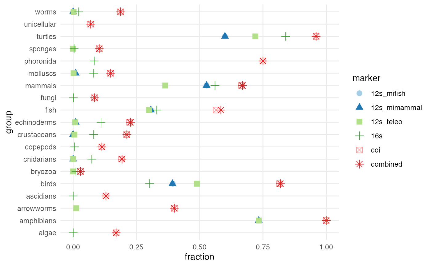

Maps

Join the gridded occurrences with the reference species lists and calculate completeness by group and cell:

grid_markers <- gridded_occurrences %>%
  select(h3, species, group) %>%
  left_join(reference_species %>% select(marker, species), by = "species") %>%
  group_by(h3, group) %>%
  mutate(
    group_species = n_distinct(species),
    group_species_in_reference = n_distinct(species[!is.na(marker)])
  ) %>%
  group_by(h3, group, group_species, group_species_in_reference, marker) %>%
  summarize(
    group_marker_species = n_distinct(species)
  ) %>%
  ungroup()

grid_markers %>% filter(group == "fish" & h3 == "82000ffffffffff")
#> # A tibble: 6 × 6
#>   h3      group group_species group_species_in_ref…¹ marker group_marker_species
#>   <chr>   <chr>         <int>                  <int> <chr>                 <int>
#> 1 82000f… fish             44                     39 12s_m…                   32
#> 2 82000f… fish             44                     39 12s_m…                   32
#> 3 82000f… fish             44                     39 12s_t…                   33
#> 4 82000f… fish             44                     39 16s                      31
#> 5 82000f… fish             44                     39 coi                      39
#> 6 82000f… fish             44                     39 NA                        5
#> # ℹ abbreviated name: ¹​group_species_in_reference

land <- rnaturalearth::ne_countries(scale = "medium", returnclass = "sf")

make_map <- function(selected_group, selected_marker) {
  map_grid <- grid_markers %>%
    filter(group == selected_group & marker == selected_marker) %>%
    mutate(fraction = group_marker_species / group_species) %>%
    select(h3, group_species, group_marker_species, fraction) %>%
    mutate(geometry = h3jsr::cell_to_polygon(h3)) %>%
    st_as_sf() %>%
    st_wrap_dateline(options = c("WRAPDATELINE=YES", "DATELINEOFFSET=180"))
  
  ggplot() +
    geom_sf(data = map_grid, aes(fill = fraction)) +
    geom_sf(data = land, fill = "white", color = "black") +
    scale_fill_gradientn(colours = c("#7d1500", "#da4325", "#eca24e", "#e7e2bc", "#5cc3af", "#0a6265"), values = seq(0, 1, 0.2)) +
    coord_sf(crs = st_crs("+proj=robin +lon_0=0 +x_0=0 +y_0=0 +ellps=WGS84 +datum=WGS84 +units=m +no_defs")) +
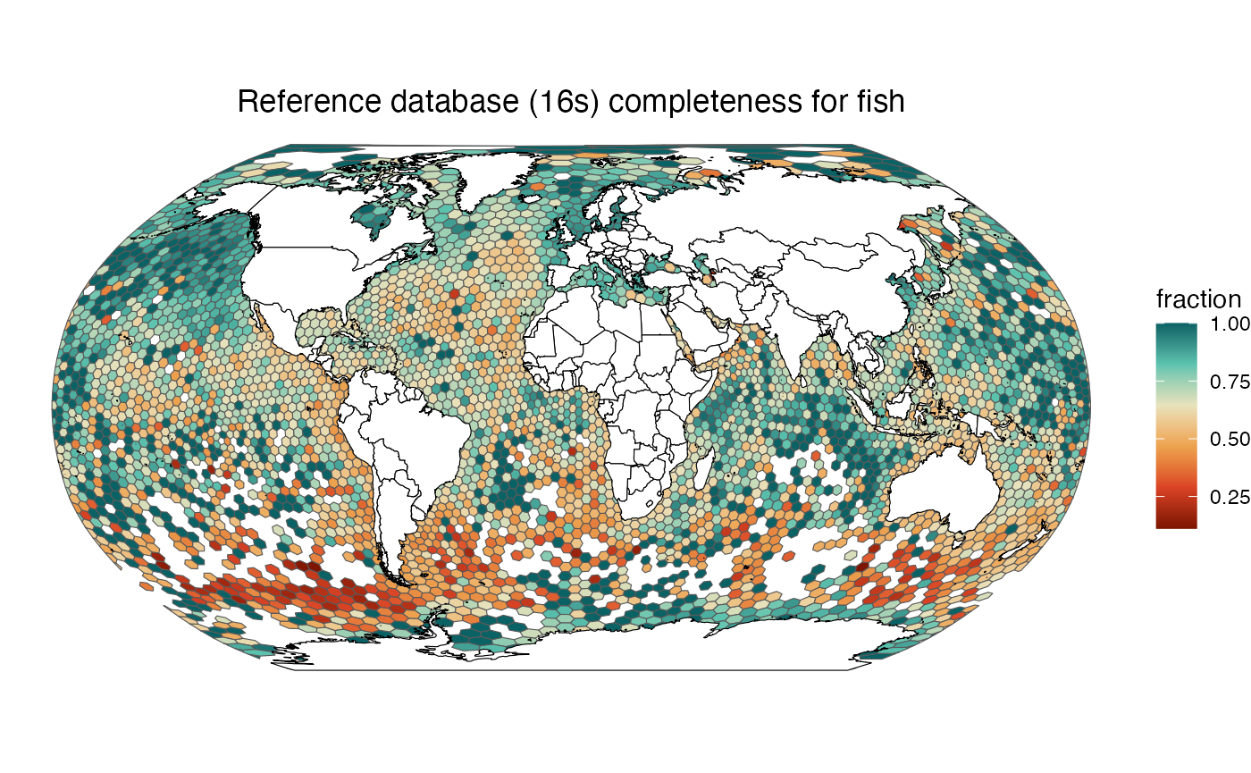
    ggtitle(glue("Reference database ({selected_marker}) completeness for {selected_group}")) +
    theme_void() +
    theme(plot.title = element_text(hjust = 0.5))
}

make_map("fish", "12s_mifish")

make_map("fish", "12s_mimammal")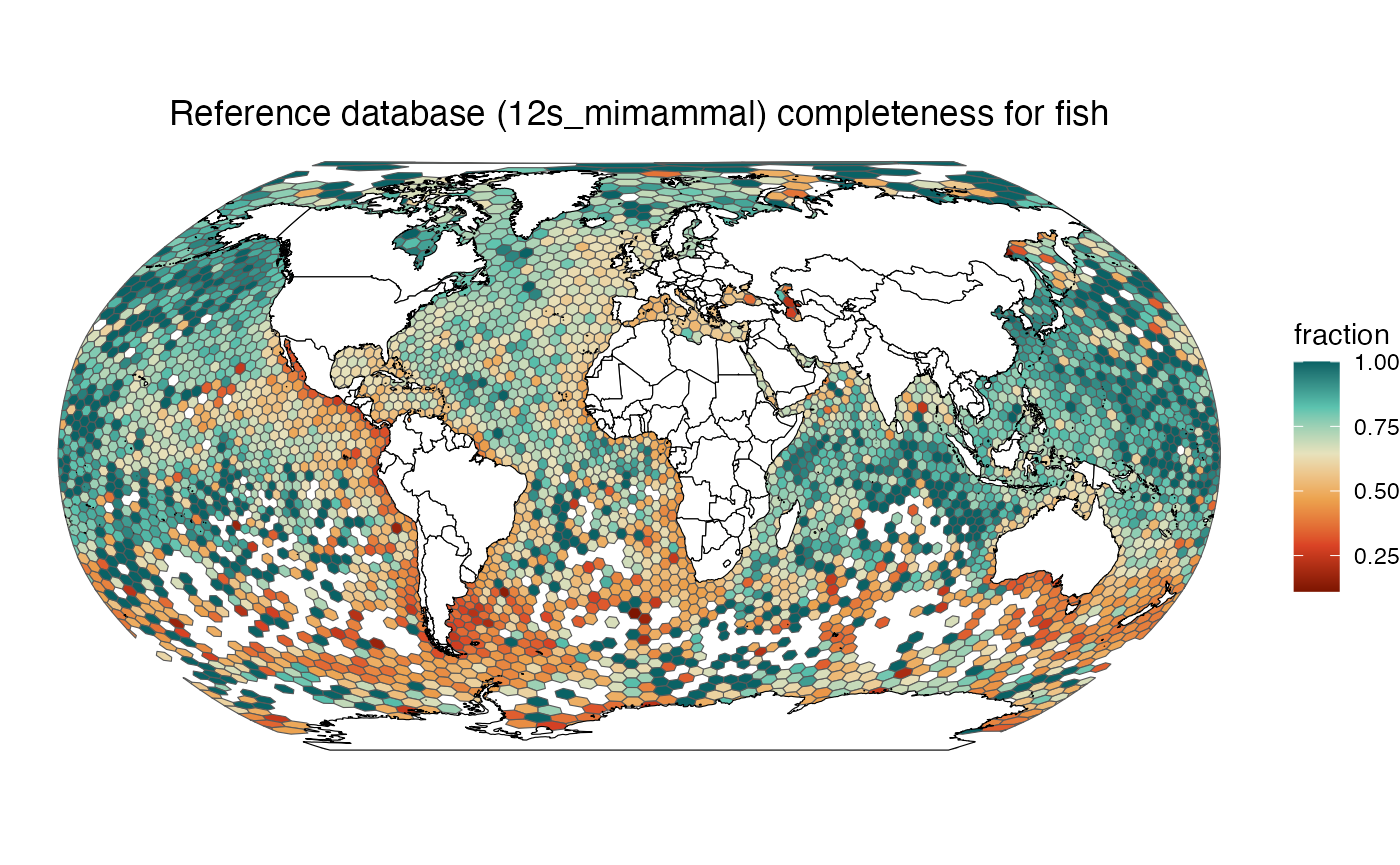

make_map("fish", "12s_teleo")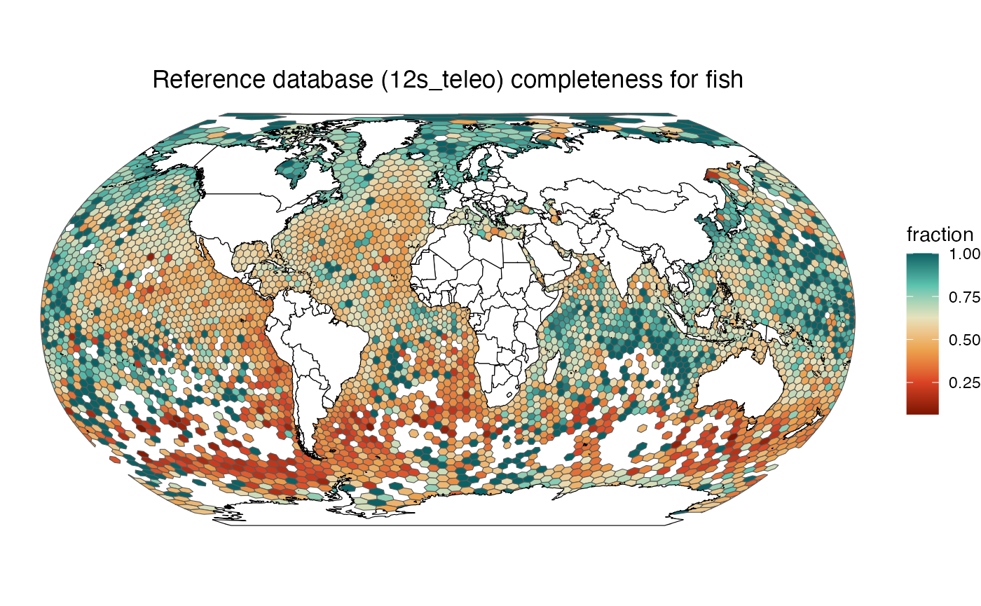

make_map("fish", "coi")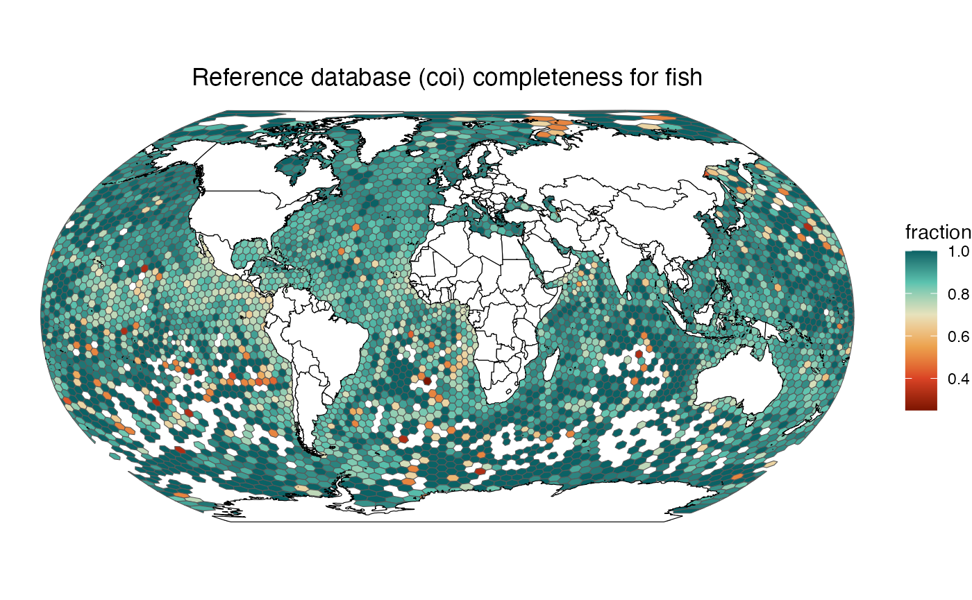

make_map("fish", "16s")