Species sequence identity in the eDNA Expeditions reference databases • ednagaps

Dependencies

library(ednagaps)
library(dplyr)
library(Biostrings)
library(msa)
library(ggmsa)
library(ggdist)
library(ggplot2)
library(glue)
library(purrr)

Reference databases

Reference database creation is documented at https://github.com/iobis/edna-reference-databases, and reference databases were downloaded to reference_databases from the LifeWatch server using:

rsync -avrm --partial --progress --include='*/' --include='*pga_tax.tsv' --include='*pga_taxa.tsv' --include='*pga_taxon.tsv' --exclude='*' ubuntu@lfw-ds001-i035.i.lifewatch.dev:/home/ubuntu/data/databases/ ./reference_databases
rm -r ./reference_databases/silva*

reference_databases <- list(
  "12s_mimammal" = list(
    taxa = "~/Desktop/edna-reference-databases/12s_ncbi_mimammal_pga_taxa.tsv",
    sequences = "~/Desktop/edna-reference-databases/12s_ncbi_mimammal_pga.fasta"
  ),
  "12s_mifish" = list(
    taxa = "~/Desktop/edna-reference-databases/12s_ncbi_mifish_pga_taxa.tsv",
    sequences = "~/Desktop/edna-reference-databases/12s_ncbi_mifish_pga.fasta"
  ),
  "12s_teleo" = list(
    taxa = "~/Desktop/edna-reference-databases/12s_ncbi_teleo_pga_taxa.tsv",
    sequences = "~/Desktop/edna-reference-databases/12s_ncbi_teleo_pga.fasta"
  ),
  "coi" = list(
    taxa = "~/Desktop/edna-reference-databases/coi_ncbi_pga_taxa.tsv",
    sequences = "~/Desktop/edna-reference-databases/coi_ncbi_pga.fasta"
  ),
  "16s" = list(
    taxa = "~/Desktop/edna-reference-databases/16s_ncbi_pga_taxa.tsv",
    sequences = "~/Desktop/edna-reference-databases/16s_ncbi_pga.fasta"
  )
)

We use this function from the ednagaps package to generate WoRMS aligned species lists by marker. We need accepted WoRMS taxonomy to reliably determine if sequences are from the same species or not.

generate_reference_species(reference_databases)

Analysis

First read the reference databases, and join the accepted WoRMS taxonomy. Sequences without an accepted WoRMS name and a marine or brackish flag are not retained.

input_taxonomy <- read_input_taxonomy() %>%
  filter(rank == "Species" & (isMarine == 1 | isBrackish == 1)) %>% 
  select(input, phylum, class, order, family, genus, species = scientificname)
#> Warning: One or more parsing issues, call `problems()` on your data frame for details,
#> e.g.:
#>   dat <- vroom(...)
#>   problems(dat)

db <- read_reference_databases(reference_databases) %>% 
  filter(!is.na(species)) %>% 
  select(marker, seqid, sequence, input = species) %>% 
  inner_join(input_taxonomy, by = "input", keep = FALSE)
#>  ■■■■■■■■■■■■■■■■■■■               60% |  ETA:  2s
#>  ■■■■■■■■■■■■■■■■■■■■■■■■■         80% |  ETA: 27s

ggplot() +
  geom_boxplot(data = db, aes(x = marker, y = nchar(sequence)), alpha = 0.5) +
  facet_wrap(~marker, scales = "free") +
  ggtitle("Sequence length")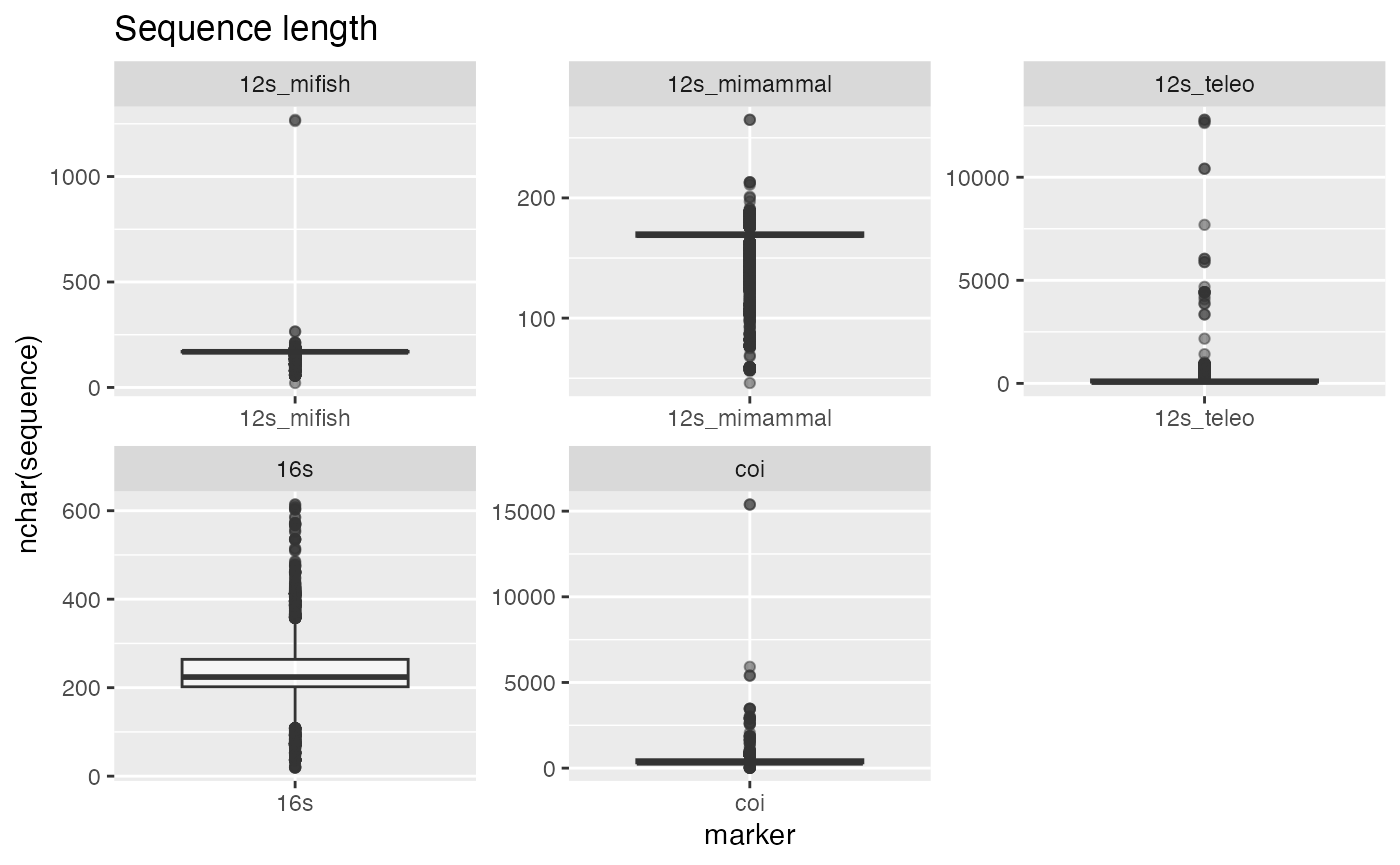

The function below writes a set of sequences to fasta, performs a blast of all sequences against all sequences, and returns the results. The results are filtered to remove self-alignments, and the query coverage is calculated.

align <- function(sequences) {
  sequence_lengths <- data.frame(query_acc_ver = sequences$seqid, sequence_length = nchar(sequences$sequence))
  seqinr::write.fasta(as.list(sequences$sequence), file.out = "sequences.fasta", names = sequences$seqid, as.string = TRUE)
  result <- tryCatch({
    pipe(glue("blastn -query sequences.fasta -subject sequences.fasta -word_size 11 -dust no -outfmt 6")) %>%
      read.table() %>%
      setNames(c("query_acc_ver", "subject_acc_ver", "perc_identity", "alignment_length", "mismatches", "gap_opens", "q_start", "q_end", "s_start", "s_end", "evalue", "bit_score"))
  }, error = function(err) {
    message(err)
  })
  file.remove("sequences.fasta")
  result %>%
    filter(query_acc_ver != subject_acc_ver) %>%
    mutate(combined = paste0(pmin(query_acc_ver, subject_acc_ver), "_", pmax(query_acc_ver, subject_acc_ver))) %>%
    distinct(combined, .keep_all = TRUE) %>% 
    left_join(sequence_lengths, by = "query_acc_ver") %>% 
    mutate(query_cover = (q_end - q_start + 1) / sequence_length * 100)
}

Now process sequences for each marker and each genus. We select a maximum of 10 sequences per species. Results are written to a storr cache per marker.

max_sequences_per_species <- 10

for (selected_marker in names(reference_databases)) {
  message(selected_marker)
  st <- storr::storr_rds(glue("~/Desktop/temp/storr_{selected_marker}"))

  for (selected_genus in sort(unique(db$genus))) {
    message(selected_genus)
    if (!st$exists(selected_genus)) {
      sequences_genus <- db %>% 
        filter(marker == selected_marker & genus == selected_genus) %>% 
        group_by(species) %>% 
        slice_sample(n = max_sequences_per_species) %>% 
        arrange(genus, species)
      if (nrow(sequences_genus) < 2) next()
      genus_results <- align(sequences_genus) %>%
        select(query_acc_ver, subject_acc_ver, perc_identity, alignment_length, query_cover) %>%
        left_join(sequences_genus %>% select(seqid, species1 = species), by = c("query_acc_ver" = "seqid")) %>% 
        left_join(sequences_genus %>% select(seqid, species2 = species), by = c("subject_acc_ver" = "seqid")) %>% 
        mutate(same_species = species1 == species2) %>%
        mutate(genus = selected_genus)
      st$set(selected_genus, genus_results)
    }
  }
}

Finally, we read the results from the storr cache and visualize the results, filtering for a minimum query cover of 90%. These are sequence identities within species versus between species of the same genus.

min_query_cover <- 90

results <- map(names(reference_databases), function(selected_marker) {
  storr_path <- glue("~/Desktop/temp/storr_{selected_marker}")
  if (!file.exists(storr_path)) return(NULL)
  st <- storr::storr_rds(storr_path)
  map(st$list(), st$get) %>% 
    bind_rows() %>% mutate(marker = selected_marker) 
}) %>% bind_rows()

ggplot(results %>% filter(query_cover >= min_query_cover)) +
  stat_halfeye(aes(x = same_species, y = perc_identity, fill = same_species), justification = -0.2, .width = 0, adjust = 30) +
  stat_boxplot(aes(x = same_species, y = perc_identity, fill = same_species), width = 0.2, outlier.size = 0.1, outliers = TRUE) +
  theme_minimal() +
  scale_fill_brewer(palette = "Set1") +
  facet_wrap(~marker) +
  theme(legend.position = "none")

We can now calculate some cutoff values for clustering based on the within species sequence identity. This shows that the cutoff should be lower for COI than for 12S.

results %>%
  filter(query_cover >= min_query_cover & same_species) %>%
  group_by(marker) %>%
  summarise(
    p1 = quantile(perc_identity, 0.01),
    p5 = quantile(perc_identity, 0.05),
    p10 = quantile(perc_identity, 0.10),
    p15 = quantile(perc_identity, 0.15),
    p20 = quantile(perc_identity, 0.20)
  )
#> # A tibble: 5 × 6
#>   marker          p1    p5   p10   p15   p20
#>   <chr>        <dbl> <dbl> <dbl> <dbl> <dbl>
#> 1 12s_mifish    86.8  94.6  97.7  98.8  99.4
#> 2 12s_mimammal  86.5  94.5  97.7  98.8  99.4
#> 3 12s_teleo     87.1  95.1  98.2  98.4  99.4
#> 4 16s           86.4  92.7  96.1  97.7  98.5
#> 5 coi           80.9  88.8  94.8  97.4  98.4